Quickstart: WaveOrder

# Install WaveOrder and dependencies
# This includes torch, iohub, matplotlib, and other required packages
import subprocess
import sys

# Check if running in Colab
try:
    import google.colab  # noqa: F401
    IN_COLAB = True
except ImportError:
    IN_COLAB = False

if IN_COLAB:
    # IMPORTANT: This notebook requires the quickstart-notebook branch
    # Once merged to main, update this to: "waveorder>=2.0.0"
    subprocess.check_call([
        sys.executable, "-m", "pip", "install", "-q",
        "git+https://github.com/mehta-lab/waveorder.git@quickstart-notebook",
        "iohub>=0.2.0", "matplotlib"
    ])
    print("✓ Installed waveorder (quickstart-notebook branch) and dependencies")

# embedded_data = ""

from pathlib import Path

# Download demo data file
!gdown https://drive.google.com/uc?id=1btFRQVkKo4Di6_hVa8iz3r5UuHAfXOhe
demo_file = Path("demo_fov.npz")

Output:

Downloading...
From: https://drive.google.com/uc?id=1btFRQVkKo4Di6_hVa8iz3r5UuHAfXOhe
To: /content/demo_fov.npz
100% 3.97M/3.97M [00:00<00:00, 24.7MB/s]

# === Imports ===
import numpy as np
import torch
import matplotlib.pyplot as plt

# WaveOrder imports
from waveorder import util
from waveorder.models import isotropic_thin_3d

# Set style
plt.style.use('default')
np.random.seed(42)
torch.manual_seed(42)

# === Helper Functions ===


def load_embedded_demo_data(demo_file=Path("demo_fov.npz"), embedded_data=""):
    """Extract embedded demo dataset

    If using your own data, make sure to set the EMBEDDED_DATA
    variable to your data in string format.
    """
    import base64

    if demo_file.exists():
        print(f"✓ Demo data already exists: {demo_file}")
        return demo_file

    if EMBEDDED_DATA:
      print("Extracting embedded demo data...")
      # Decode and write to file
      data_bytes = base64.b64decode(EMBEDDED_DATA)
      demo_file.write_bytes(data_bytes)
      print(f"✓ Extracted demo data: {demo_file}")
      print(f"  Size: {demo_file.stat().st_size / 1024 / 1024:.1f} MB")
      return demo_file
    else:
      print("𐄂 Please set the EMBEDDED_DATA variable.")
      return None


def load_demo_data(npz_file):
    """Load demo data from .npz file"""
    data = np.load(npz_file)
    zyx_data = data['data']
    scale = data['scale']
    z_scale, y_scale, x_scale = scale[-3:]

    print("✓ Loaded data")
    print(f"  Shape: {zyx_data.shape}")
    print(
        f"  Scale: z={z_scale:.3f}, y={y_scale:.3f}, "
        f"x={x_scale:.3f} µm/pixel"
    )
    print(f"  Data range: [{zyx_data.min():.3f}, {zyx_data.max():.3f}]")

    return zyx_data, z_scale, y_scale, x_scale


def run_reconstruction(zyx_tile, recon_args):
    """
    Run WaveOrder phase reconstruction

    Parameters
    ----------
    zyx_tile : torch.Tensor
        3D image stack (Z, Y, X)
    recon_args : dict
        Dictionary of optical parameters

    Returns
    -------
    yx_phase_recon : torch.Tensor
        2D reconstructed phase image
    """
    tf_args = recon_args.copy()
    Z, _, _ = zyx_tile.shape

    # Create z-position array accounting for offset
    tf_args["z_position_list"] = (
        torch.arange(Z) - (Z // 2) + recon_args["z_offset"]
    ) * recon_args["z_scale"]
    tf_args.pop("z_offset")
    tf_args.pop("z_scale")

    # Core reconstruction: calculate transfer functions
    tf_abs, tf_phase = isotropic_thin_3d.calculate_transfer_function(
        **tf_args
    )

    # Calculate singular value decomposition
    system = isotropic_thin_3d.calculate_singular_system(tf_abs, tf_phase)

    # Apply inverse transfer function (Tikhonov-regularized)
    _, yx_phase_recon = isotropic_thin_3d.apply_inverse_transfer_function(
        zyx_tile, system, regularization_strength=1e-2
    )

    return yx_phase_recon


def compute_midband_power(
    yx_array, NA_det, lambda_ill, pixel_size, band=(0.1, 0.2)
):
    """
    Compute power in mid-band spatial frequencies

    This serves as an image quality metric:
    - Higher mid-band power = sharper, better-focused image
    - Lower mid-band power = blurry or defocused image
    """
    _, _, fxx, fyy = util.gen_coordinate(yx_array.shape, pixel_size)
    frr = torch.tensor(np.sqrt(fxx**2 + fyy**2))
    xy_abs_fft = torch.abs(torch.fft.fftn(yx_array))
    cutoff = 2 * NA_det / lambda_ill
    mask = torch.logical_and(
        frr > cutoff * band[0], frr < cutoff * band[1]
    )
    return torch.sum(xy_abs_fft[mask])


def prepare_optimizer(optimizable_params):
    """Prepare PyTorch parameters and optimizer"""
    optimization_params = {}
    optimizer_config = []

    for name, (enabled, initial, lr) in optimizable_params.items():
        if enabled:
            param = torch.nn.Parameter(
                torch.tensor([initial], device="cpu"), requires_grad=True
            )
            optimization_params[name] = param
            optimizer_config.append({"params": [param], "lr": lr})

    optimizer = torch.optim.Adam(optimizer_config)
    return optimization_params, optimizer


def optimize_reconstruction(
    zyx_tile, recon_args, optimizable_params, num_iterations=20
):
    """
    Optimize optical parameters to maximize mid-band frequency power

    Returns
    -------
    yx_recon : torch.Tensor
        Optimized reconstruction
    final_params : dict
        Dictionary of optimized parameter values
    history : list
        List of (loss, params) at each iteration
    """
    optimization_params, optimizer = prepare_optimizer(
        optimizable_params
    )
    history = []

    print(f"Optimizing for {num_iterations} iterations...")

    for step in range(num_iterations):
        # Update recon_args with current parameter values
        for name, param in optimization_params.items():
            recon_args[name] = param

        # Run reconstruction
        yx_recon = run_reconstruction(zyx_tile, recon_args)

        # Compute loss (negative mid-band power, since we're minimizing)
        loss = -compute_midband_power(
            yx_recon,
            NA_det=0.15,
            lambda_ill=recon_args["wavelength_illumination"],
            pixel_size=recon_args["yx_pixel_size"],
            band=(0.1, 0.2),
        )

        # Backward pass and optimizer step
        loss.backward()
        optimizer.step()
        optimizer.zero_grad()

        # Store history
        param_values = {
            name: param.item() for name, param in optimization_params.items()
        }
        history.append((loss.item(), param_values.copy()))

        # Print progress every iteration
        print(f"  Iteration {step+1:2d}: Loss = {loss.item():.2e}")

    print("✓ Optimization complete!")

    # Extract final parameters
    final_params = {
        name: param.item() for name, param in optimization_params.items()
    }

    return yx_recon.detach(), final_params, history


def get_central_crop(image, crop_fraction=0.5):
    """Extract central crop from image"""
    h, w = image.shape[-2:]
    ch, cw = int(h * crop_fraction), int(w * crop_fraction)
    y0, x0 = (h - ch) // 2, (w - cw) // 2
    return image[..., y0:y0 + ch, x0:x0 + cw]


print("✓ Setup complete")

# Load embedded demo data
demo_file = load_embedded_demo_data()
zyx_data, z_scale, y_scale, x_scale = load_demo_data(demo_file)

# To use your own data, comment out the above lines and load your data here:
# zyx_data = your_data_array  # Shape: (Z, Y, X)
# z_scale, y_scale, x_scale = 0.5, 0.108, 0.108  # Your pixel sizes in µm

# Visualize the raw data
Z, Y, X = zyx_data.shape

fig, axes = plt.subplots(1, 3, figsize=(15, 4))

# Z-projection (maximum intensity)
axes[0].imshow(np.max(zyx_data, axis=0), cmap='gray')
axes[0].set_title('Max Projection (Z)', fontweight='bold')
axes[0].axis('off')

# Middle slice
mid_z = Z // 2
axes[1].imshow(zyx_data[mid_z], cmap='gray')
axes[1].set_title(
    f'Middle Slice (z={mid_z*z_scale:.1f}µm)', fontweight='bold'
)
axes[1].axis('off')

# Z-profile through center
center_y, center_x = Y // 2, X // 2
z_positions = np.arange(Z) * z_scale
axes[2].plot(z_positions, zyx_data[:, center_y, center_x], 'k-', linewidth=2)
axes[2].set_xlabel('Z position (µm)')
axes[2].set_ylabel('Intensity (a.u.)')
axes[2].set_title('Intensity Profile (center)', fontweight='bold')
axes[2].grid(True, alpha=0.3)

plt.tight_layout()
plt.show()

print(f"\nData characteristics:")
print(f"  • Z-slices: {Z} (spanning {Z*z_scale:.1f} µm)")
print(f"  • FOV: {Y}×{X} pixels ({Y*y_scale:.1f}×{X*x_scale:.1f} µm)")

Output:

✓ Demo data already exists: demo_fov.npz
✓ Loaded data
  Shape: (9, 512, 512)
  Scale: z=25.000, y=1.300, x=1.300 µm/pixel
  Data range: [983.000, 24835.000]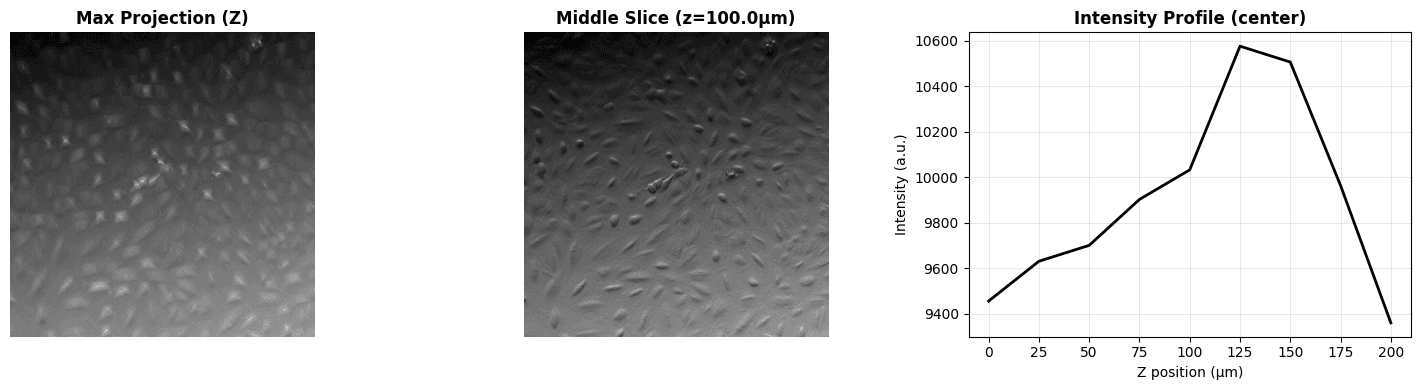

Output:

Data characteristics:
  • Z-slices: 9 (spanning 225.0 µm)
  • FOV: 512×512 pixels (665.6×665.6 µm)

# Fixed optical parameters (from microscope specifications)
FIXED_PARAMS = {
    "wavelength_illumination": 0.450,  # 450 nm (blue LED)
    "index_of_refraction_media": 1.0,  # Air
    "invert_phase_contrast": True,  # Invert for proper phase sign
}

# Initial guesses for optical parameters (nominal values)
INITIAL_PARAMS = {
    "z_offset": 0.0,  # No defocus offset (assumed)
    "numerical_aperture_detection": 0.15,  # Detection NA (from spec)
    "numerical_aperture_illumination": 0.1,  # Illumination NA (estimated)
    "tilt_angle_zenith": 0.1,  # Tilt from vertical (radians)
    "tilt_angle_azimuth": 260 * np.pi / 180,  # Tilt direction (radians)
}

# Display parameters
print("Optical System Parameters")
print("=" * 70)
print(f"{'Parameter':<40} {'Value':<15} {'Unit':<10}")
print("-" * 70)
print(
    f"{'Illumination wavelength':<40} "
    f"{FIXED_PARAMS['wavelength_illumination']:<15.3f} {'µm':<10}"
)
print(
    f"{'Refractive index':<40} "
    f"{FIXED_PARAMS['index_of_refraction_media']:<15.1f} {'':<10}"
)
print(
    f"{'Defocus offset':<40} "
    f"{INITIAL_PARAMS['z_offset']:<15.2f} {'µm':<10}"
)
print(
    f"{'Detection NA':<40} "
    f"{INITIAL_PARAMS['numerical_aperture_detection']:<15.3f} {'':<10}"
)
print(
    f"{'Illumination NA':<40} "
    f"{INITIAL_PARAMS['numerical_aperture_illumination']:<15.3f} {'':<10}"
)
print(
    f"{'Tilt zenith':<40} "
    f"{INITIAL_PARAMS['tilt_angle_zenith']:<15.3f} {'rad':<10}"
)
print(
    f"{'Tilt azimuth':<40} "
    f"{INITIAL_PARAMS['tilt_angle_azimuth']:<15.3f} {'rad':<10}"
)
print("=" * 70)

Output:

Optical System Parameters
======================================================================
Parameter                                Value           Unit      
----------------------------------------------------------------------
Illumination wavelength                  0.450           µm        
Refractive index                         1.0                       
Defocus offset                           0.00            µm        
Detection NA                             0.150                     
Illumination NA                          0.100                     
Tilt zenith                              0.100           rad       
Tilt azimuth                             4.538           rad       
======================================================================

# Convert data to PyTorch tensor
zyx_tensor = torch.tensor(zyx_data, dtype=torch.float32, device="cpu")

# Prepare reconstruction arguments
recon_args = FIXED_PARAMS.copy()
for name, value in INITIAL_PARAMS.items():
    recon_args[name] = torch.tensor(
        [value], dtype=torch.float32, device="cpu"
    )

recon_args["yx_shape"] = zyx_tensor.shape[1:]
recon_args["yx_pixel_size"] = y_scale
recon_args["z_scale"] = z_scale

print("Running initial reconstruction...")
initial_recon = run_reconstruction(zyx_tensor, recon_args)
print(f"✓ Reconstruction complete. Output shape: {initial_recon.shape}")

# Visualize initial reconstruction
initial_crop = get_central_crop(initial_recon, crop_fraction=0.5)

fig, axes = plt.subplots(1, 2, figsize=(12, 5))

# Real space (central 50% crop)
im0 = axes[0].imshow(initial_crop.detach().numpy(), cmap='gray')
axes[0].set_title('Phase (Real Space)', fontweight='bold')
axes[0].axis('off')
plt.colorbar(im0, ax=axes[0], label='Phase (radians)', fraction=0.046)

# Fourier space (power spectrum)
fft_recon = torch.fft.fftshift(torch.fft.fftn(initial_recon))
power_spectrum = torch.log10(torch.abs(fft_recon)**2 + 1e-10)

im1 = axes[1].imshow(power_spectrum.detach().numpy(), cmap='gray')
axes[1].set_title('Power Spectrum (Fourier Space)', fontweight='bold')
axes[1].axis('off')
plt.colorbar(im1, ax=axes[1], label='log₁₀(Power)', fraction=0.046)

plt.suptitle(
    'Initial Reconstruction (Nominal Parameters)',
    fontsize=14,
    fontweight='bold',
    y=1.02
)
plt.tight_layout()
plt.show()

phase_np = initial_recon.detach().numpy()
print(f"\nReconstruction statistics:")
print(f"  • Phase range: [{phase_np.min():.3f}, {phase_np.max():.3f}] rad")
print(f"  • Phase std: {phase_np.std():.3f} rad")

Output:

Running initial reconstruction...
✓ Reconstruction complete. Output shape: torch.Size([512, 512])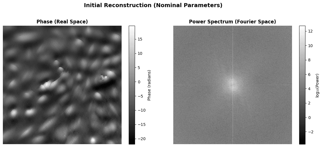

Output:

Reconstruction statistics:
  • Phase range: [-21.946, 176.058] rad
  • Phase std: 27.157 rad

# Define which parameters to optimize and their learning rates
OPTIMIZABLE_PARAMS = {
    # (optimize?, initial_value, learning_rate)
    "z_offset": (True, 0.0, 0.01),
    "numerical_aperture_detection": (True, 0.15, 0.001),
    "numerical_aperture_illumination": (True, 0.1, 0.001),
    "tilt_angle_zenith": (True, 0.1, 0.005),
    "tilt_angle_azimuth": (True, 260 * np.pi / 180, 0.001),
}

NUM_ITERATIONS = 20

print("Optimization Configuration")
print("=" * 70)
print(
    f"{'Parameter':<40} {'Optimize?':<12} {'Initial':<12} {'LR':<10}"
)
print("-" * 70)
for name, (optimize, initial, lr) in OPTIMIZABLE_PARAMS.items():
    print(
        f"{name:<40} {'Yes' if optimize else 'No':<12} "
        f"{initial:<12.4f} {lr:<10.5f}"
    )
print(f"\nIterations: {NUM_ITERATIONS}")
print("=" * 70)

Output:

Optimization Configuration
======================================================================
Parameter                                Optimize?    Initial      LR        
----------------------------------------------------------------------
z_offset                                 Yes          0.0000       0.01000   
numerical_aperture_detection             Yes          0.1500       0.00100   
numerical_aperture_illumination          Yes          0.1000       0.00100   
tilt_angle_zenith                        Yes          0.1000       0.00500   
tilt_angle_azimuth                       Yes          4.5379       0.00100   

Iterations: 20
======================================================================

# Run optimization
optimized_recon, final_params, history = optimize_reconstruction(
    zyx_tensor,
    recon_args,
    OPTIMIZABLE_PARAMS,
    num_iterations=NUM_ITERATIONS,
)

# Visualize optimization progress
losses = [h[0] for h in history]
param_names = list(history[0][1].keys())

fig, axes = plt.subplots(2, 3, figsize=(15, 8))
axes = axes.flatten()

# Plot loss
axes[0].plot(losses, 'k-', linewidth=2)
axes[0].set_xlabel('Iteration')
axes[0].set_ylabel('Loss')
axes[0].set_title('Optimization Loss', fontweight='bold')
axes[0].grid(True, alpha=0.3)

# Plot each parameter
initial_param_values = {
    name: val[1] for name, val in OPTIMIZABLE_PARAMS.items() if val[0]
}

for idx, param_name in enumerate(param_names):
    param_history = [h[1][param_name] for h in history]
    initial_val = initial_param_values[param_name]
    final_val = final_params[param_name]

    axes[idx + 1].plot(
        param_history, 'b-', linewidth=2, label='Optimized'
    )
    axes[idx + 1].axhline(
        initial_val, color='gray', linestyle='--', label='Initial'
    )
    axes[idx + 1].set_xlabel('Iteration')
    axes[idx + 1].set_ylabel(param_name.replace('_', ' '))
    axes[idx + 1].set_title(
        param_name.replace('_', ' '), fontsize=10, fontweight='bold'
    )
    axes[idx + 1].grid(True, alpha=0.3)
    axes[idx + 1].legend(fontsize=8)

    # Add change annotation
    change = final_val - initial_val
    change_pct = 100 * change / initial_val if initial_val != 0 else 0
    textstr = f'Δ={change:+.4f}\n({change_pct:+.1f}%)'
    axes[idx + 1].text(
        0.05,
        0.95,
        textstr,
        transform=axes[idx + 1].transAxes,
        verticalalignment='top',
        fontsize=8,
        bbox={'boxstyle': 'round', 'facecolor': 'wheat', 'alpha': 0.5},
    )

plt.suptitle('Optimization Progress', fontsize=14, fontweight='bold')
plt.tight_layout()
plt.show()

# Print parameter changes
print("\nParameter Changes:")
print("=" * 85)
print(
    f"{'Parameter':<35} {'Initial':<12} {'Final':<12} "
    f"{'Change':<12} {'% Change':<12}"
)
print("-" * 85)
for param_name in param_names:
    initial_val = initial_param_values[param_name]
    final_val = final_params[param_name]
    change = final_val - initial_val
    change_pct = 100 * change / initial_val if initial_val != 0 else 0
    print(
        f"{param_name:<35} {initial_val:<12.4f} {final_val:<12.4f} "
        f"{change:+12.4f} {change_pct:+12.1f}%"
    )
print("=" * 85)

# Check convergence by looking at recent loss changes
recent_losses = [h[0] for h in history[-5:]]
loss_changes = [
    abs(recent_losses[i] - recent_losses[i - 1])
    for i in range(1, len(recent_losses))
]
avg_recent_change = np.mean(loss_changes) if loss_changes else 0
relative_change = (
    avg_recent_change / abs(recent_losses[-1])
    if recent_losses[-1] != 0
    else 0
)

print("\nConvergence Analysis:")
print("-" * 85)
print(f"Average loss change (last 5 iterations): {avg_recent_change:.2e}")
print(f"Relative change: {relative_change*100:.3f}%")

if relative_change > 0.01:  # Still changing by more than 1%
    print(
        "\n⚠ Note: Parameters have not fully converged "
        "after 20 iterations."
    )
    print(
        "   The loss is still decreasing, suggesting further "
        "optimization could improve results."
    )
    print("\n   To improve convergence, try:")
    print("   • Increase NUM_ITERATIONS to 50 or 100")
    print(
        "   • Adjust learning rates in OPTIMIZABLE_PARAMS "
        "(try reducing by half)"
    )
    print(
        "   • Run this optimization cell again to continue "
        "from current parameters"
    )
else:
    print("\n✓ Parameters appear to have converged (loss changes < 1%)")
print("=" * 85)

Output:

Optimizing for 20 iterations...
  Iteration  1: Loss = -1.36e+07
  Iteration  2: Loss = -1.41e+07
  Iteration  3: Loss = -1.46e+07
  Iteration  4: Loss = -1.51e+07
  Iteration  5: Loss = -1.55e+07
  Iteration  6: Loss = -1.59e+07
  Iteration  7: Loss = -1.63e+07
  Iteration  8: Loss = -1.66e+07
  Iteration  9: Loss = -1.68e+07
  Iteration 10: Loss = -1.71e+07
  Iteration 11: Loss = -1.73e+07
  Iteration 12: Loss = -1.74e+07
  Iteration 13: Loss = -1.75e+07
  Iteration 14: Loss = -1.77e+07
  Iteration 15: Loss = -1.78e+07
  Iteration 16: Loss = -1.80e+07
  Iteration 17: Loss = -1.82e+07
  Iteration 18: Loss = -1.84e+07
  Iteration 19: Loss = -1.87e+07
  Iteration 20: Loss = -1.89e+07
✓ Optimization complete!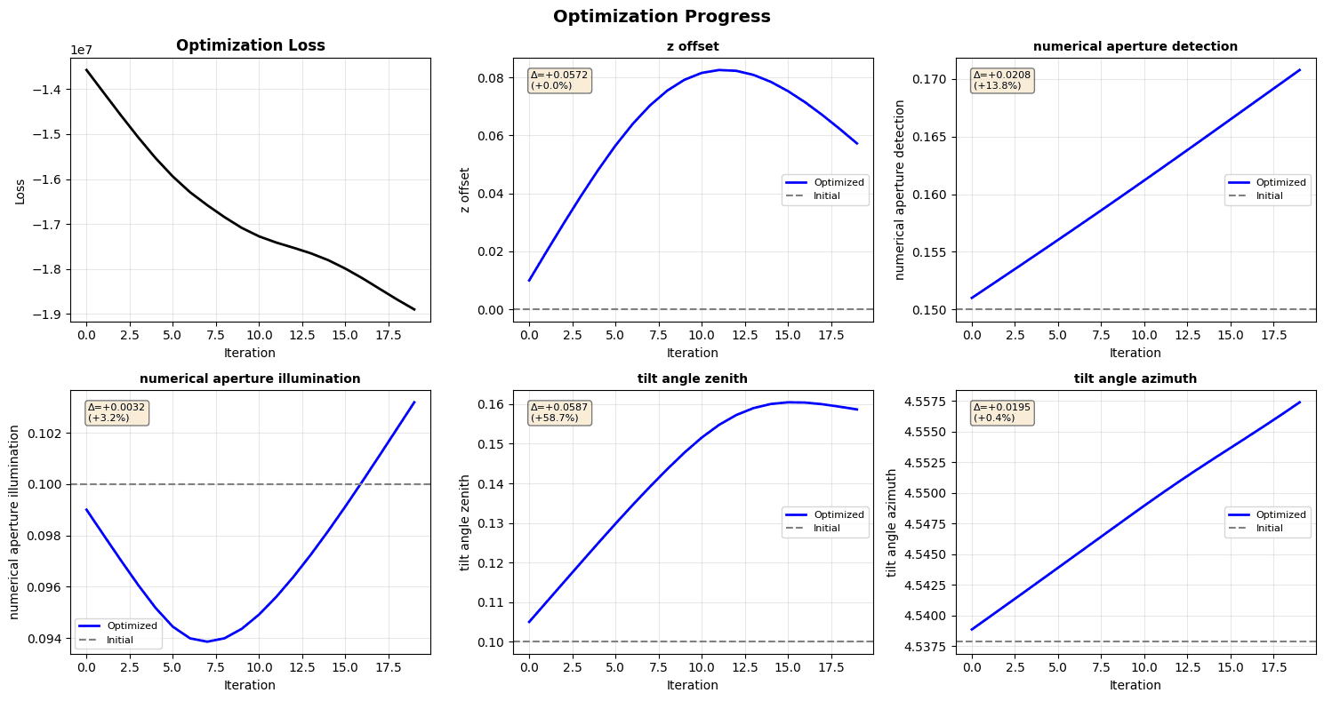

Output:

Parameter Changes:
=====================================================================================
Parameter                           Initial      Final        Change       % Change    
-------------------------------------------------------------------------------------
z_offset                            0.0000       0.0572            +0.0572         +0.0%
numerical_aperture_detection        0.1500       0.1708            +0.0208        +13.8%
numerical_aperture_illumination     0.1000       0.1032            +0.0032         +3.2%
tilt_angle_zenith                   0.1000       0.1587            +0.0587        +58.7%
tilt_angle_azimuth                  4.5379       4.5574            +0.0195         +0.4%
=====================================================================================

Convergence Analysis:
-------------------------------------------------------------------------------------
Average loss change (last 5 iterations): 2.27e+05
Relative change: 1.203%

⚠ Note: Parameters have not fully converged after 20 iterations.
   The loss is still decreasing, suggesting further optimization could improve results.

   To improve convergence, try:
   • Increase NUM_ITERATIONS to 50 or 100
   • Adjust learning rates in OPTIMIZABLE_PARAMS (try reducing by half)
   • Run this optimization cell again to continue from current parameters
=====================================================================================

# Visualize optimized reconstruction
optimized_crop = get_central_crop(optimized_recon, crop_fraction=0.5)

fig, axes = plt.subplots(1, 2, figsize=(12, 5))

# Real space (central 50% crop)
im0 = axes[0].imshow(optimized_crop.detach().numpy(), cmap='gray')
axes[0].set_title('Phase (Real Space)', fontweight='bold')
axes[0].axis('off')
plt.colorbar(im0, ax=axes[0], label='Phase (radians)', fraction=0.046)

# Fourier space (power spectrum)
fft_optimized = torch.fft.fftshift(torch.fft.fftn(optimized_recon))
power_optimized = torch.log10(torch.abs(fft_optimized)**2 + 1e-10)

im1 = axes[1].imshow(power_optimized.detach().numpy(), cmap='gray')
axes[1].set_title('Power Spectrum (Fourier Space)', fontweight='bold')
axes[1].axis('off')
plt.colorbar(im1, ax=axes[1], label='log₁₀(Power)', fraction=0.046)

plt.suptitle(
    'Optimized Reconstruction', fontsize=14, fontweight='bold', y=1.02
)
plt.tight_layout()
plt.show()

phase_np = optimized_recon.detach().numpy()
print(f"\nReconstruction statistics:")
print(f"  • Phase range: [{phase_np.min():.3f}, {phase_np.max():.3f}] rad")
print(f"  • Phase std: {phase_np.std():.3f} rad")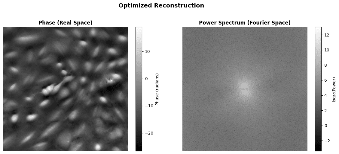

Output:


Reconstruction statistics:
  • Phase range: [-26.610, 156.208] rad
  • Phase std: 31.206 rad

# Side-by-side comparison
initial_crop = get_central_crop(initial_recon, crop_fraction=0.5)
optimized_crop = get_central_crop(optimized_recon, crop_fraction=0.5)

# Use same color scale for both
vmin = min(initial_crop.min().item(), optimized_crop.min().item())
vmax = max(initial_crop.max().item(), optimized_crop.max().item())

fig, axes = plt.subplots(1, 3, figsize=(15, 5))

# Initial
im0 = axes[0].imshow(
    initial_crop.detach().numpy(), cmap='gray', vmin=vmin, vmax=vmax
)
axes[0].set_title('Initial', fontweight='bold')
axes[0].axis('off')

# Optimized
im1 = axes[1].imshow(
    optimized_crop.detach().numpy(), cmap='gray', vmin=vmin, vmax=vmax
)
axes[1].set_title('Optimized', fontweight='bold')
axes[1].axis('off')

# Difference
diff_crop = optimized_crop - initial_crop
im2 = axes[2].imshow(diff_crop.detach().numpy(), cmap='gray')
axes[2].set_title('Difference (Optimized - Initial)', fontweight='bold')
axes[2].axis('off')

# Add colorbars
plt.colorbar(im0, ax=axes[0], label='Phase (rad)', fraction=0.046)
plt.colorbar(im1, ax=axes[1], label='Phase (rad)', fraction=0.046)
plt.colorbar(im2, ax=axes[2], label='Δ Phase (rad)', fraction=0.046)

plt.suptitle(
    'Reconstruction Comparison (Central 50% Crop)',
    fontsize=14,
    fontweight='bold',
    y=0.98
)
plt.tight_layout()
plt.show()

# Compute comparison metrics
initial_midband = compute_midband_power(
    initial_recon,
    final_params['numerical_aperture_detection'],
    FIXED_PARAMS['wavelength_illumination'],
    y_scale,
    band=(0.1, 0.2)
)
optimized_midband = compute_midband_power(
    optimized_recon,
    final_params['numerical_aperture_detection'],
    FIXED_PARAMS['wavelength_illumination'],
    y_scale,
    band=(0.1, 0.2)
)

improvement = (
    (optimized_midband - initial_midband) / initial_midband * 100
)

print("\nComparison Metrics:")
print("=" * 70)
print(f"Mid-band power (initial):    {initial_midband.item():.2e}")
print(f"Mid-band power (optimized):  {optimized_midband.item():.2e}")
print(f"Improvement:                 {improvement.item():+.1f}%")
print()
print(
    f"Phase std (initial):         {initial_recon.std().item():.4f} rad"
)
print(
    f"Phase std (optimized):       {optimized_recon.std().item():.4f} rad"
)
print()
diff = optimized_recon - initial_recon
print(
    f"Max absolute difference:     "
    f"{torch.abs(diff).max().item():.4f} rad"
)
print(
    f"Mean absolute difference:    "
    f"{torch.abs(diff).mean().item():.4f} rad"
)
print("=" * 70)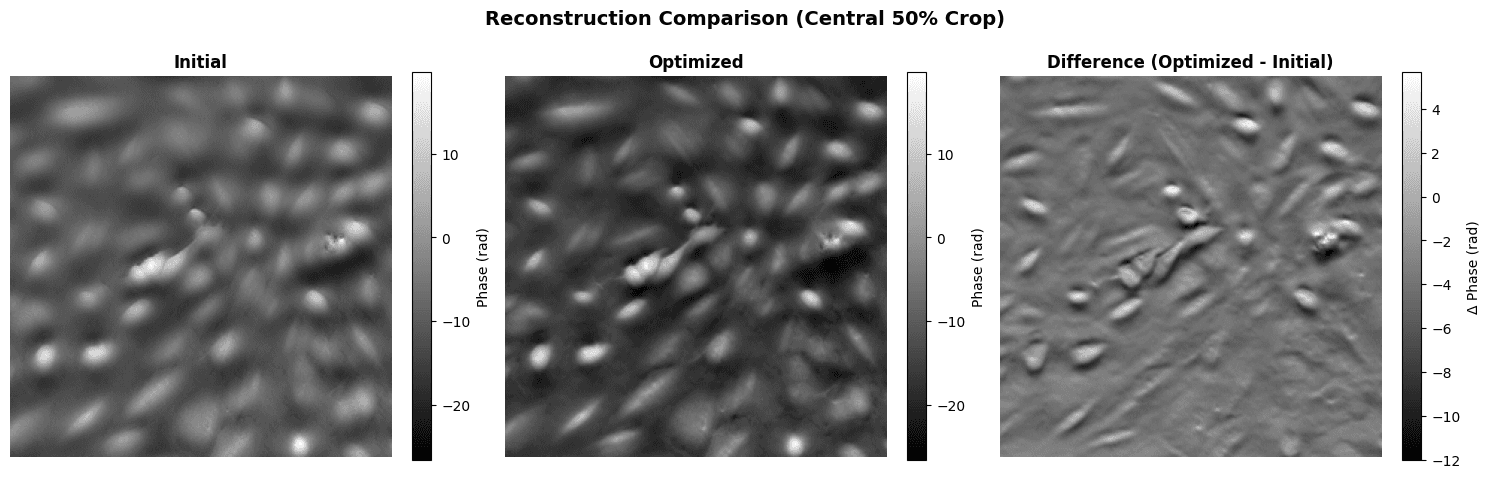

Output:

Comparison Metrics:
======================================================================
Mid-band power (initial):    1.34e+07
Mid-band power (optimized):  1.79e+07
Improvement:                 +34.2%

Phase std (initial):         27.1568 rad
Phase std (optimized):       31.2064 rad

Max absolute difference:     30.0756 rad
Mean absolute difference:    5.6141 rad
======================================================================