scGenePT Perturbation Prediction Tutorial

Last Updated: [12/04/2024] This notebook offers examples of how to use trained scGenePT models in inference mode for perturbation prediction. It uses models fine-tuned on the Norman dataset [1] and offers examples of predicting post-perturbation expression responses for single gene perturbations: POU3F2, CDKN1B and gene combinations: SAMD1+ZBTB1. Models have not been evaluated on multiple gene combination perturbation responses, so behavior is unknown.

Model : scGenePT is a collection of single-cell models for perturbation prediction. It leverages the scGPT [2] foundation model for scRNAseq data by injecting language embeddings at the gene level into the model architecture. The language gene embeddings are obtained by embedding gene level information from different knowledge sources using LLMs. The knowledge sources used include NCBI gene descriptions, UniProt protein Summaries for protein coding genes - as inspired by the genePT [3] approach - and GO (Gene Ontology) Gene Molecular Annotations, across three different axes: Molecular Function, Biological Process and Cellular Component. The model variations available are:

scGenePT_NCBI = scGPT + NCBI Gene Card Summaries
scGenePT_NCBI+UniProt = scGPT + NCBI Gene Card Summaries + UniProt Protein Summaries
scGenePT_GO-F = scGPT + GO Molecular Functions Annotations
scGenePT_GO-C = scGPT + GO Cellular Components Annotations
scGenePT_GO-P = scGPT + GO Biological Processes Annotations
scGenePT+GO-all = scGPT + GO_F + GO_C + GO_P

In this tutorial, we will focus on comparing scGenePT_GO-C and scGenePT_NCBI+UniProt models.

Dataset: The Norman Dataset [1] is a CRISPR perturb-seq dataset containing single and two-gene perturbations. We use a processed version of the dataset that contains 105 single and 131 two-gene combinations perturbations coming from 91k observations. Cells in the dataset are log-normalized and filtered to the top 5000 highly variable genes. Models in ths notebook are trained on the train split of the dataset. We offer examples of:

performing inference on the test split of the Norman dataset
performing inference on a random control sample and on a new anndata file

Hardware Requirements: We strongly recommend running this notebook on a GPU instance. It should run on a CPU as well, but it will be much slower.

The notebook is structured and offers the following examples:

Perturbation prediction
- Loading the Norman dataset
- Loading a trained scGenePT model
Plotting the top 20 Differentially Expressed Genes post-perturbation
Perturbation prediction on NumPy arrays holding control samples
Perturbation prediction on AnnData files

Setup

We start by installing the required packages needed to run the notebook, as well as adding the needed data. Note that this section might take a few minutes to run:

%%capture [--no-stderr]
!pip -q install torch==2.1.2 torch_geometric==2.5.3 torchdata==0.7.1 torchmetrics==1.4.0.post0 packaging==24.1 numpy==1.26.4 scgpt awscli

!git clone https://github.com/czi-ai/scGenePT.git

from pathlib import Path
def initialize_folder_structure(models_dir, models, dataset):
  models_finetuned = models_dir / "finetuned"
  model_embeddings = models_dir / "gene_embeddings"
  model_embeddings_annotations = models_dir / "gene_embeddings" / "gene_annotations"
  models_finetuned.mkdir(parents=True, exist_ok=True)
  for model in models:
    model_dir = models_finetuned / model / dataset
    model_dir.mkdir(parents=True, exist_ok=True)
  model_embeddings.mkdir(parents=True, exist_ok=True)
  model_embeddings_annotations.mkdir(parents=True, exist_ok=True)

# This creates the required folder structure needed for the data
initialize_folder_structure(Path('scGenePT/models'), ['scgpt', 'scgenept_go_c', 'scgenept_ncbi+uniprot'], "norman")

Model and Data

The trained models can be downloaded from S3:

dataset_name = 'norman' # this can also be replaced with adamson, but the model files need to be updated accordingly throughout the notebook

# Download the Gene Embeddings
!aws s3 cp --no-sign-request s3://czi-scgenept-public/models/gene_embeddings/GO_C_gene_embeddings-gpt3.5-ada-concat.pickle scGenePT/models/gene_embeddings/
!aws s3 cp --no-sign-request s3://czi-scgenept-public/models/gene_embeddings/NCBI+UniProt_embeddings-gpt3.5-ada.pkl  scGenePT/models/gene_embeddings/

# Download the trained scGenePT models
!aws s3 sync --no-sign-request s3://czi-scgenept-public/models/finetuned/scgpt/{dataset_name}/ scGenePT/models/finetuned/scgpt/{dataset_name}/
!aws s3 sync --no-sign-request s3://czi-scgenept-public/models/finetuned/scgenept_go_c/norman/ scGenePT/models/finetuned/scgenept_go_c/{dataset_name}/
!aws s3 sync --no-sign-request s3://czi-scgenept-public/models/finetuned/scgenept_ncbi+uniprot/{dataset_name}/ scGenePT/models/finetuned/scgenept_ncbi+uniprot/{dataset_name}/

Note that in this tutorial, we focus on comparing scGenePT_GO-C and scGenePT_NCBI+UniProt models, but all the other model variations can be downloaded in a similar way. The s3 links follow the structure:

s3://czi-scgenept-public/models/finetuned/{scgenept_model_name}/{dataset_name}

So if you would like to download other model variations, you have to change the scgenept_model_name, and if you want to a model trained on a different dataset, you need to change the dataset_name.

For instance, to download a scGenePT_GO-P model trained on Adamson, you would run:

!aws s3 sync --no-sign-request s3://czi-scgenept-public/models/finetuned/scgenept_go_p/adamson/ scGenePT/models/finetuned/scgenept_go_p/adamson/

Alternatively, you can mount all the assets at once - including all models and gene embeddings - by running the command below. Note that this will take a few min, as it will download ~10GB of data:

!aws s3 sync --no-sign-request s3://czi-scgenept-public/models scGenePT/models

Your folder structure should now look something like:

- models
    - pretrained
        - scgpt/vocab.json
    - gene_embeddings
        - GO_C_gene_embeddings-gpt3.5-ada-concat.pickle
        - NCBI+UniProt_embeddings-gpt3.5-ada.pkl
        - gene_annotations
            - gene_ontology_C.csv
            - gene_ontology_P.csv
            - gene_ontology_F.csv
            - NCBI_summary_of_genes.json
            - NCBI_UniProt_summary_of_genes.json
    - finetuned
        - scgpt/norman/best_model_rnd_seed_42_concat.pt
        - scgenept_go_c/norman/best_model_gpt3.5_ada_rnd_seed_42_concat.pt
        - scgenept_ncbi+uniprot/norman/best_model_gpt3.5_ada_rnd_seed_42_concat.pt
- tutorials
    - scgenept_tutorial.ipynb

%%capture [--no-stderr]
import sys
sys.path.insert(1, 'scGenePT')

from train import load_dataloader
from utils.data_loading import *
from models.scGenePT import *
import matplotlib.pyplot as plt
from gears.inference import evaluate, compute_metrics, deeper_analysis, non_dropout_analysis
import scanpy as sc
import pickle as pkl

1. Perturbation Prediction using a trained scGenePT model

Load dataset

We start by inspecting the Norman dataset that the models were trained on. The dataloaders we used for training used a pre-processed version of Norman from GEARS [3]. Models in this notebook have been finetuned on the train split of this dataset. We can look at the AnnData file that contains all the data used for training/validation and testing. We will inspect the splits in a later section.

!aws s3 cp --no-sign-request s3://czi-scgenept-public/training_data/{dataset_name}_pert_data_adata.h5ad.gz scGenePT/tutorials/{dataset_name}_pert_data_adata.h5ad.gz
!gzip -d scGenePT/tutorials/{dataset_name}_pert_data_adata.h5ad.gz

pert_adata = sc.read_h5ad(f'scGenePT/tutorials/{dataset_name}_pert_data_adata.h5ad')

The code below can be used to get the same data directly from GEARS dataloaders. Note that it need ~20GB of memory and will time out on a T4 Google Collab instance. But it will run on an instance with larger RAM memory.

from gears import PertData

# Download the Pre-processed Norman dataset directly from GEARS
pert_data = PertData('./data')
pert_data = load_dataloader(dataset_name, batch_size, eval_batch_size, split = 'simulation')
train_loader = pert_data.dataloader['train_loader']
val_loader = pert_data.dataloader['val_loader']
test_loader = pert_data.dataloader['test_loader']

pert_adata = pert_data.adata
pert_data_subgroup = pert_data.subgroup

Dataset Exploration

This AnnData object contains gene expression counts and additional information about the cell observations:

pert_adata

# Output

    AnnData object with n_obs × n_vars = 91205 × 5045
        obs: 'condition', 'cell_type', 'dose_val', 'control', 'condition_name'
        var: 'gene_name'
        uns: 'non_dropout_gene_idx', 'non_zeros_gene_idx', 'rank_genes_groups_cov_all', 'top_non_dropout_de_20', 'top_non_zero_de_20'
        layers: 'counts'

The gene expression counts are stored in pert_adata.X, where each entry (i, j) corresponds to the gene expression counts of gene j in row i.

pert_adata.X # 902105 cells, 5045 genes

The pert_adata.obs file contains information about the different perturbation conditions applied to the data stored in .X. For instance, below we can see examples of 1-gene perturbations: TSC22D1+ctrl, MAML2+ctrl, etc, examples of 2-gene perturbations: KLF1+MAP2K6, CEBPE+RUNX1T1, and examples of control samples. Each of the conditions corresponds to gene expression counts stored in .X.

pert_adata.obs # perturbation conditions applied to the 902105 cells

# Output:
                           condition  cell_type  dose_val  control         condition_name
          cell_barcode
    AAACCTGAGGCATGTG-1  TSC22D1+ctrl       A549       1+1        0  A549_TSC22D1+ctrl_1+1
    AAACCTGAGGCCCTTG-1   KLF1+MAP2K6       A549       1+1        0   A549_KLF1+MAP2K6_1+1
    AAACCTGCACGAAGCA-1          ctrl       A549         1        1            A549_ctrl_1
    AAACCTGCAGACGTAG-1 CEBPE+RUNX1T1       A549       1+1        0 A549_CEBPE+RUNX1T1_1+1
    AAACCTGCAGCCTTGG-1    MAML2+ctrl       A549       1+1        0    A549_MAML2+ctrl_1+1
                   ...           ...        ...       ...      ...                    ...
    TTTGTCAGTCATGCAT-8  RHOXF2BB+SET       A549       1+1        0  A549_RHOXF2BB+SET_1+1
    TTTGTCATCAGTACGT-8    FOXA3+ctrl       A549       1+1        0    A549_FOXA3+ctrl_1+1
    TTTGTCATCCACTCCA-8    CELF2+ctrl       A549       1+1        0    A549_CELF2+ctrl_1+1
    TTTGTCATCCCAACGG-8   BCORL1+ctrl       A549       1+1        0   A549_BCORL1+ctrl_1+1
    TTTGTCATCTGGCGAC-8   MAP4K3+ctrl       A549       1+1        0   A549_MAP4K3+ctrl_1+1
    91205 rows × 5 columns

The pert_adata.var gives us the set of genes:

print(f'There are {len(pert_adata.var)} number of genes present in the dataset.')
pert_adata.var.head() # the names of the 5045 genes

# Output:

    There are 5045 number of genes present in the dataset.

                        gene_name
            gene_id
    ENSG00000239945  RP11-34P13.8
    ENSG00000223764   RP11-54O7.3
    ENSG00000187634        SAMD11
    ENSG00000187642         PERM1
    ENSG00000188290          HES4

Load trained scGenePT models

In this section, we show examples of loading multiple scGenePT models for prediction in order to compare them. All the models under the scGenePT Model Zoo can be found under GitHub repo and the trained model weights under s3://czi-scgenept-public/models.

Here, we load the following models

scGPT = scGPT
scGenePT_NCBI+UniProt = scGPT + NCBI Gene Card Summaries + UniProt Protein Summaries
scGenePT_GO-C = scGPT + GO Cellular Components Annotations

Note that models are assumed to be under the models/finetuned/{dataset_name}/{model_type}/ folder.

def load_trained_scgenept_model(adata, model_type, models_dir, model_location, device, verbose = False):
    embs_to_include = get_embs_to_include(model_type)
    vocab_file = models_dir + 'pretrained/scgpt/vocab.json'
    vocab, gene_ids, dataset_genes, gene2idx = match_genes_to_scgpt_vocab_from_adata(vocab_file, adata, SPECIAL_TOKENS)
    ntokens = len(vocab)  # size of vocabulary
    genept_embs, genept_emb_type, genept_emb_dim, found_genes_genept = initialize_genept_embeddings(embs_to_include, dataset_genes, vocab, model_type, models_dir)
    go_embs_to_include, go_emb_type, go_emb_dim, found_genes_go = initialize_go_embeddings(embs_to_include, dataset_genes, vocab, model_type, models_dir)

    # we disable flash attention for inference for simplicity
    use_fast_transformer = False

    model = scGenePT(
        ntoken=ntokens,
        d_model=EMBSIZE,
        nhead=NHEAD,
        d_hid=D_HID,
        nlayers=NLAYERS,
        nlayers_cls=N_LAYERS_CLS,
        n_cls=N_CLS,
        vocab=vocab,
        n_perturbagens=2,
        dropout=0.0,
        pad_token=PAD_TOKEN,
        pad_value=PAD_VALUE,
        pert_pad_id=PERT_PAD_ID,
        use_fast_transformer=use_fast_transformer,
        embs_to_include = embs_to_include,
        genept_embs = genept_embs,
        genept_emb_type = genept_emb_type,
        genept_emb_size = genept_emb_dim,
        go_embs_to_include = go_embs_to_include,
        go_emb_type = go_emb_type,
        go_emb_size = go_emb_dim
    )

    pretrained_params = torch.load(model_location, weights_only=True, map_location = device)
    if not use_fast_transformer:
        pretrained_params = {
            k.replace("Wqkv.", "in_proj_"): v for k, v in pretrained_params.items()
        }

    model.load_state_dict(pretrained_params)

    if verbose:
        print(model)
    model.to(device)
    return model, gene_ids

device = torch.device("cuda" if torch.cuda.is_available() else "cpu")
print(f'Using device {device}')

# Mapping from model name to the name of the model file model weights are saved
model_name2model_variation = {'scgpt' : 'best_model_seed_42.pt',
                    'scgenept_ncbi+uniprot_gpt' : 'best_model_gpt3.5_ada_rnd_seed_42.pt',
                    'scgenept_go_c_gpt_concat' : 'best_model_gpt3.5_ada_rnd_seed_42_concat.pt'}
# Names of the scGenePT models to load. Note that these have to match the keys in the model_name2model_variation dict
models = ['scgpt', 'scgenept_go_c_gpt_concat', 'scgenept_ncbi+uniprot_gpt']

# To load all the models, uncomment this code and download the specific models from S3 using:
# !aws s3://czi-scgenept-public/models/finetuned/{scgenept_model_name}/{dataset_name} scGenePT/models/finetuned/{scgenept_model_name}/{dataset_name}
# model_name2model_variation = {'scgpt' : 'best_model_seed_42.pt',
#                     'scgenept_ncbi_gpt' : 'best_model_gpt3.5_ada_rnd_seed_42.pt',
#                     'scgenept_ncbi+uniprot_gpt' : 'best_model_gpt3.5_ada_rnd_seed_42.pt',
#                     'scgenept_go_c_gpt_concat' : 'best_model_gpt3.5_ada_rnd_seed_42_concat.pt',
#                     'scgenept_go_f_gpt_concat' : 'best_model_gpt3.5_ada_rnd_seed_42_concat.pt',
#                     'scgenept_go_p_gpt_concat' : 'best_model_gpt3.5_ada_rnd_seed_42_concat.pt',
#                     'scgenept_go_all_gpt_concat' : 'best_model_gpt3.5_ada_rnd_seed_42_concat.pt'}
# models = ['scgpt',  'scgenept_go_c_gpt_concat', 'scgenept_go_p_gpt_concat', 'scgenept_go_f_gpt_concat', 'scgenept_go_all_gpt_concat', 'scgenept_ncbi_gpt', 'scgenept_ncbi+uniprot_gpt']
trained_models = {}

# Location of where the pretrained scGPT model and gene embeddings are located
pretrained_scgpt_model_dir = 'scGenePT/models/'

for model_name in models:
    print(f"Now loading a {model_name} model ... ")
    print('=' * 30)
    model_filename = model_name2model_variation[model_name]
    if model_name != 'scgpt':
        model_prefix = ''.join(model_name.split('_gpt')[:-1])
    else:
        model_prefix = model_name
    model_location =  f'scGenePT/models/finetuned/{model_prefix}/{dataset_name}/{model_filename}'
    model, gene_ids =  load_trained_scgenept_model(pert_adata, model_name, pretrained_scgpt_model_dir, model_location, device)
    print('Done!\n')
    trained_models[model_name] = model

# Output:

    Using device cuda
    Now loading a scgpt model ... 
    ==============================
    scGenePT model-type: scgpt
    match 4547/5045 genes in vocabulary of size 60697.
    Using the following embeddings:['scGPT_counts_embs', 'scGPT_token_embs']
    Done!

    Now loading a scgenept_go_c_gpt_concat model ... 
    ==============================
    scGenePT model-type: scgenept_go_c_gpt_concat
    match 4547/5045 genes in vocabulary of size 60697.
    Using c GO embs
    Matched 2945 out of 5045 genes in the GenePT-w embedding
    Using the following embeddings:['GO_token_embs_gpt_concat', 'scGPT_counts_embs', 'scGPT_token_embs']
    Done!

    Now loading a scgenept_ncbi+uniprot_gpt model ... 
    ==============================
    scGenePT model-type: scgenept_ncbi+uniprot_gpt
    match 4547/5045 genes in vocabulary of size 60697.
    Using ncbi+uniprot genept embs, embedded with gpt
    Matched 3351 out of 5045 genes in the GenePT-w embedding
    Using the following embeddings:['scGPT_counts_embs', 'scGPT_token_embs', 'genePT_token_embs_gpt']
    Done!

2. Plot the Top Differentially Expressed Genes post-perturbation

We can use the trained models to perform inference. Below, we offer an example of how to do this on the test split of the Norman dataset - this is novel data the model has not been trained on. In the following sections we offer examples of performing inference on completely new data, either in numpy or anndata form.

We explore the following scenarios and showcase how to plot the top differentially expressed genes post-perturbation for:

single-gene perturbation: predicting the effects of perturbing the POU3F2 gene and the CDKN1B gene individually. We offer examples of comparing scGPT with scGenePT_GO-C model predictions
two-gene perturbation: predicting the effect of perturbing the SAMD1+ZBTB1 genes simultaneously. We offer an example of comparing scGPT and scGenePT_NCBI+UniProt model predictions

def plot_perturbation(
    model: nn.Module, adata, query: str, model_type, color, marker, title, save_file: str = None, amp = True, pool_size: int = None
):
    import seaborn as sns
    import numpy as np
    import matplotlib.pyplot as plt

    sns.set_theme(style="ticks", rc={"axes.facecolor": (0, 0, 0, 0)}, font_scale=1.5)
    adata_ctrl = adata[adata.obs['condition'] == 'ctrl']
    gene_names = adata.var['gene_name'].to_list()

    gene2idx = {gene: idx for idx, gene in enumerate(adata.var['gene_name'])}
    cond2name = dict(adata.obs[["condition", "condition_name"]].values)
    gene_raw2id = dict(zip(adata.var.index.values, adata.var.gene_name.values))

    de_idx = [
        gene2idx[gene_raw2id[i]]
        for i in adata.uns["top_non_zero_de_20"][cond2name[query]]
    ]
    genes = [
        gene_raw2id[i] for i in adata.uns["top_non_zero_de_20"][cond2name[query]]
    ]
    truth = adata[adata.obs.condition == query].X.toarray()[:, de_idx]
    print(device)
    pred = model.pred_perturb_from_ctrl(adata_ctrl, query, gene_names, device, gene_ids, amp, pool_size).squeeze()[de_idx]
    ctrl_means = adata[adata.obs["condition"] == "ctrl"].to_df().mean()[de_idx].values

    pred = pred - ctrl_means
    truth = truth - ctrl_means

    plt.figure(figsize=[16.5, 4.5])
    plt.title(title + '\n' + query)
    plt.boxplot(truth, showfliers=False, medianprops=dict(linewidth=0))

    for i in range(pred.shape[0]):
        _ = plt.scatter(i + 1, pred[i], color=color, marker=marker)

    plt.axhline(0, linestyle="dashed", color="green")

    ax = plt.gca()
    ax.xaxis.set_ticklabels(genes, rotation=90)

    plt.ylabel("Change in Gene Expression over Control", labelpad=10)
    plt.tick_params(axis="x", which="major", pad=5)
    plt.tick_params(axis="y", which="major", pad=5)
    sns.despine()

Before we perform predictions, we can explore the test split of the Norman dataset in more detail. We are interested in this split, because this is data that the model has not seen during training, so performance on this data gives us a sense of model performance on unseen data. The pert_data.subgroup object contains information about the set of perturbations present in each of the train/val/test splits. These subgroups represent the perturbations in the AnnData file pert_adata explored previously, that were used for training/validation or testing.

pert_data_subgroup = pkl.load(open(f'scGenePT/tutorials/{dataset_name}_pert_data_subgroups.pkl', 'rb'))
pert_data_subgroup.keys()

The perturbation types in the test set are split into the following categories:

unseen_single: single gene perturbations that have not been seen during training
combo_seen0: two-gene perturbations, none of the genes has been seen perturbed (individually or as part of a combination) during training
combo_seen1: two-gene perturbations, one of the genes has been seen perturbed (individually or as part of a combination) during training
combo_seen2: two-gene perturbations, both genes has been seen perturbed (individually or as part of a combination) during training

unseen_single = pert_data_subgroup['test_subgroup']['unseen_single']
combo_seen0 = pert_data_subgroup['test_subgroup']['combo_seen0']
combo_seen1 = pert_data_subgroup['test_subgroup']['combo_seen1']
combo_seen2 = pert_data_subgroup['test_subgroup']['combo_seen2']

print(f'unseen_single: {len(unseen_single)}, combo_seen0: {len(combo_seen0)}, combo_seen1: {len(combo_seen1)}, combo_seen2: {len(combo_seen2)}')

# Output:

    unseen_single: 37, combo_seen0: 9, combo_seen1: 52, combo_seen2: 18

Examples of combinations of genes where none of the genes has been seen during training:

combo_seen0

# Output:

    ['POU3F2+FOXL2',
    'ZBTB10+PTPN12',
    'CEBPB+PTPN12',
    'CBL+PTPN12',
    'RHOXF2BB+SET',
    'CDKN1C+CDKN1B',
    'CDKN1C+CDKN1A',
    'CDKN1B+CDKN1A',
    'C3orf72+FOXL2']

Single-Gene Perturbation: Predicting perturbation response for perturbing the POU3F2 gene

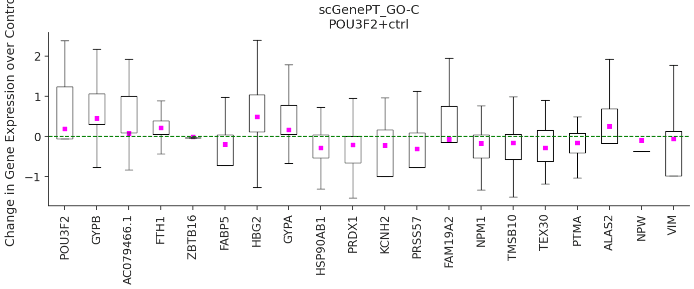
Then we can start exploring prediction on some of these perturbation categories. In the example below, we compare the perturbation prediction responses of scGPT and scGenePT_GO-C - scGPT + GO Cellular Components Annotations by perturbing the POU2F2 gene, which has not been seen perturbed during training by the model. We do this by sampling n = 300 random controls from the training dataset and taking the mean of the average prediction for each control. According to NCBI Gene Card, overexpression of the protein encoded by POU3F2 is associated with an increase in the proliferation of melanoma cells. We can see that the genes FABP5, HSP90AB1, PRDX1, NPM1, TMSB10, PTMA are all better predicted as having a negative fold change over control by scGenePTGO-C, compared to scGPT which predicts a non-significant effect.

pert = 'POU3F2+ctrl'
colors = ['blue', 'fuchsia']
marker_types = [ 'o','s']
models_to_predict = ['scgpt', 'scgenept_go_c_gpt_concat']

for model, color, marker_type, title  in zip(models_to_predict, colors, marker_types, ['scGPT', 'scGenePT_GO-C']):
    plot_perturbation(trained_models[model], pert_adata, pert, model, color, marker_type, title, amp = True, pool_size=300)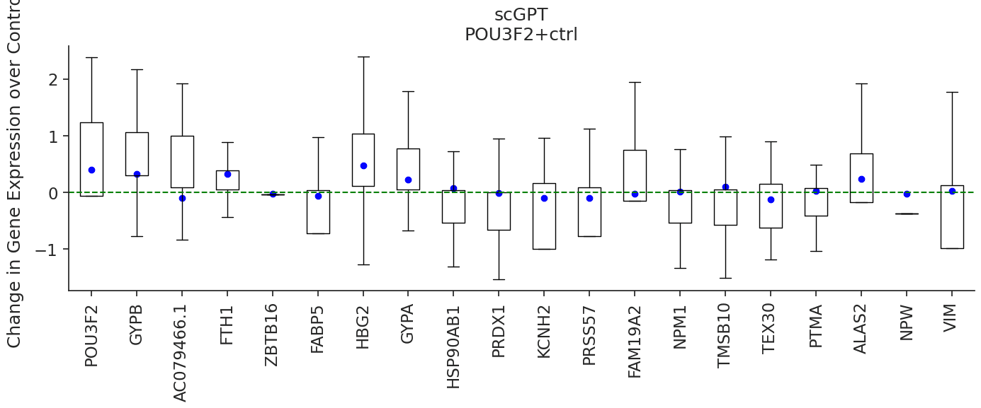

We can inspect the GO Gene Annotations that were used for this gene during training. If you don't already have the GO annotations downloaded, they can be retrieved from s3 through:

aws s3 sync --no-sign-request s3://czi-scgenept-public/models/gene_embeddings/gene_annotations/ scGenePT/models/gene_embeddings/gene_annotations/

import pandas as pd
gene_annotations_dir = 'scGenePT/models/gene_embeddings/gene_annotations/'

#GO-C Cellular Component Annotations
GO_C_annotations_df = pd.read_csv(gene_annotations_dir + 'gene_ontology_C.csv')
#GO-P Biological Process Annotations
GO_P_annotations_df = pd.read_csv(gene_annotations_dir + 'gene_ontology_P.csv')
#GO-F Molecular Function Annotations
GO_F_annotations_df = pd.read_csv(gene_annotations_dir + 'gene_ontology_F.csv')

For example, we can look at the GO-C Cellular Components annotations for the POU3F2 gene:

GO_C_annotations_df[GO_C_annotations_df['gene'] == 'POU3F2']

# Output:

                gene                                    gene_name  ontology_aspect               direct_class_label
    37738     POU3F2  POU domain, class 3, transcription factor 2                C                      nucleoplasm
    37739     POU3F2  POU domain, class 3, transcription factor 2                C                        chromatin
    37740     POU3F2  POU domain, class 3, transcription factor 2                C  transcription regulator complex

By adding the GO Cellular Component annotations, the model learns that this gene is localized mostly in: nucleoplasm, chromatin and transcription regulator complex. Similarly, it learns about the subcellular localization of the other genes. Localization of gene products in the cell plays an important role in their biological function, e.g. protein-protein interaction; regulation of gene expression, transportation of protein. This tells us that subcellular localization is helpful in being able to predict effects of perturbation of this gene.

Single-Gene Perturbation: Predicting perturbation response for perturbing the CDKN1B gene

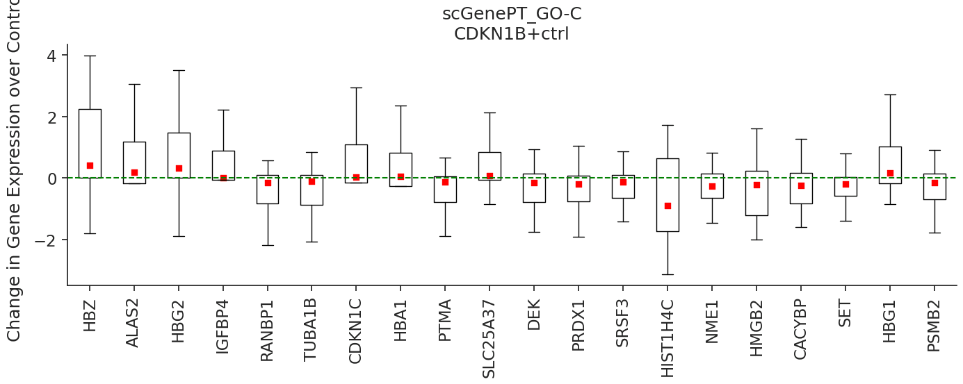
We can do this analysis for other genes as well. For example, the CDKN1B gene is another gene that has not been seen perturbed during training. According to this gene's NCBI Gene Card, mutations in this gene are associated with multiple enodcrine neoplasia type IV. We can see that scGenePTGO-C predicts HSP90AA1, PTMA, RANBP1, CKS1B, PRDX1, PHF19 and NME1 as correctly down-regulated, as opposed to scGPT which predicts either neutral effect or positive fold change. Similarly, we speculate that the model learns to incorporate cellular location information to better predict gene expression change in response to genetic perturbation.

pert = 'CDKN1B+ctrl'
colors = ['blue', 'red']
marker_types = [ 'o','s']
models_to_predict = ['scgpt', 'scgenept_go_c_gpt_concat']

for model, color, marker_type, title  in zip(models_to_predict, colors, marker_types, ['scGPT', 'scGenePT_GO-C']):
    plot_perturbation(trained_models[model], pert_adata, pert, model, color, marker_type, title, amp = True, pool_size=300)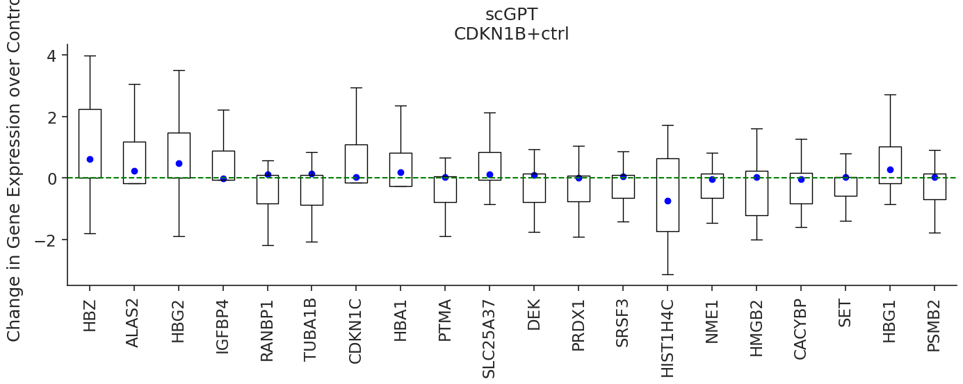

We can see that the subcellular localization annotations that the model sees during training for the CDK1NB gene are:

GO_C_annotations_df[GO_C_annotations_df['gene'] == 'CDKN1B']

# Output:

             gene                             gene_name  ontology_aspect                        direct_class_label
    72395  CDKN1B  Cyclin-dependent kinase inhibitor 1B                C                                   nucleus
    72396  CDKN1B  Cyclin-dependent kinase inhibitor 1B                C                               nucleoplasm
    72397  CDKN1B  Cyclin-dependent kinase inhibitor 1B                C                                 cytoplasm
    72398  CDKN1B  Cyclin-dependent kinase inhibitor 1B                C                                  endosome
    72399  CDKN1B  Cyclin-dependent kinase inhibitor 1B                C                                   cytosol
    72400  CDKN1B  Cyclin-dependent kinase inhibitor 1B                C  intracellular membrane-bounded organelle
    72401  CDKN1B  Cyclin-dependent kinase inhibitor 1B                C    Cul4A-RING E3 ubiquitin ligase complex

We speculate that having access to this information during training is helping the model make better predictions on the effect of perturbing this gene.

Two-gene Perturbation: Predicting perturbation response for perturbing the gene combination FOXA1+FOXL2

We can also look at effects of combination of genes. Below, we offer an example of predicting perturbation responses for the FOXA1+FOXL2 gene combination.

Note that you can experiment with different gene combinations in combo_seen0, combo_seen1, or combo_seen2

pert = 'FOXA1+FOXL2'
colors = ['blue', 'green']
marker_types = [ 'o', 's', 's']
models_to_predict = ['scgpt', 'scgenept_ncbi+uniprot_gpt']

for model, color, marker_type, title  in zip(models_to_predict, colors, marker_types, ['scGPT', 'scGenePT_NCBI+UniProt']):
    plot_perturbation(trained_models[model], pert_adata, pert, model, color, marker_type, title, amp = True, pool_size=300)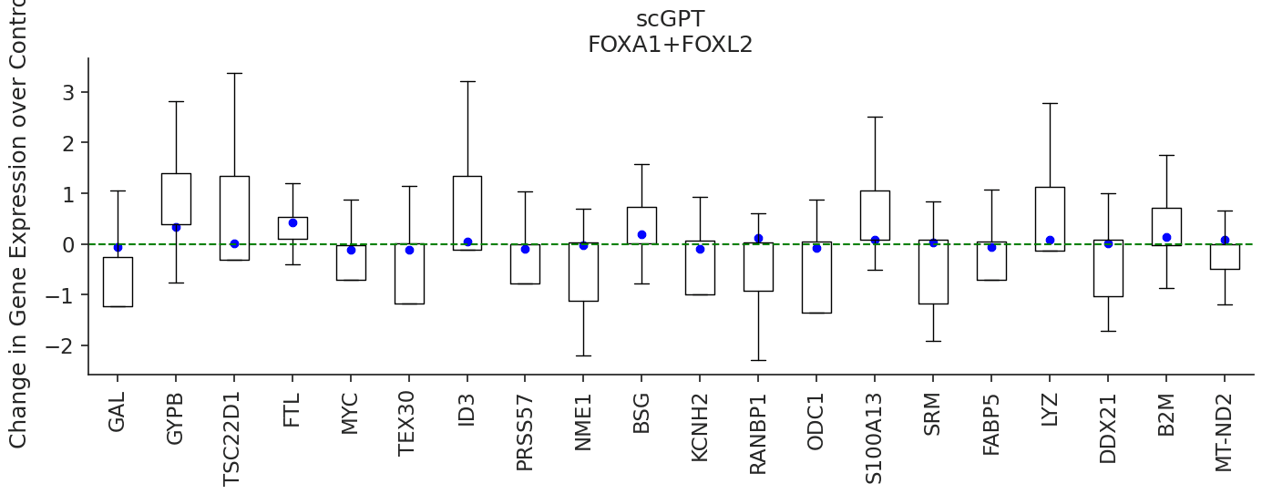

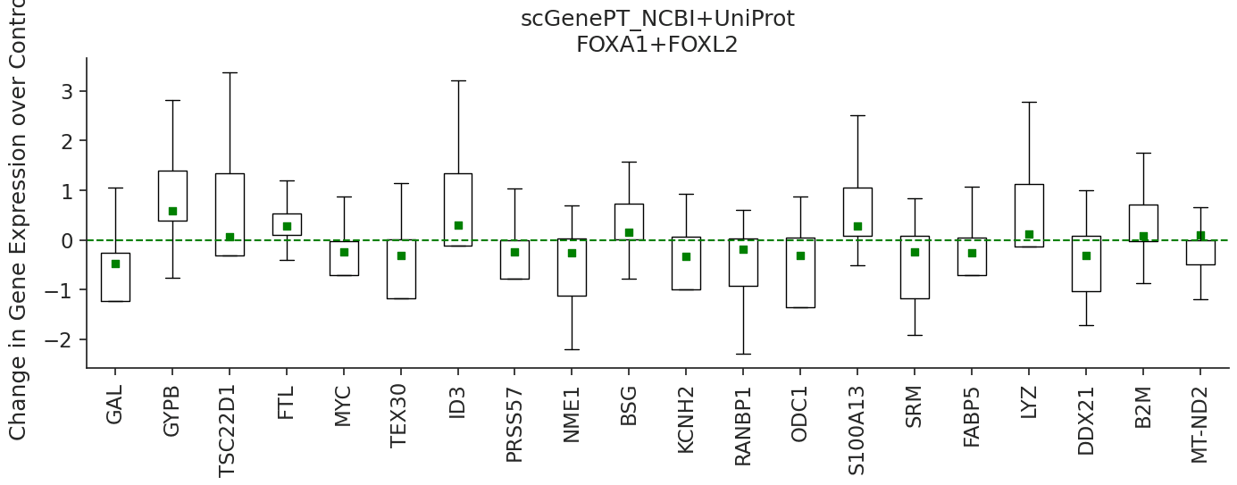
Similarly, we can look at the NCBI and UniProt annotations for the genes:

# NCBI Gene Card Annotations
NCBI_gene_card_summaries = json.load(open(gene_annotations_dir + 'NCBI_summary_of_genes.json', 'rb'))
# NCBI Gene Card + UniProt protein summaries Annotations
NCBI_UniProt_gene_card_protein_summaries = json.load(open(gene_annotations_dir + 'NCBI_UniProt_summary_of_genes.json', 'rb'))

comb_genes = pert.split('+')
for gene in comb_genes:
    print(f"Annotations for GENE: {gene}")
    print('='*30)
    print(f"NCBI Gene Card Summary: {NCBI_gene_card_summaries[gene]}")
    print('\n')
    print(f"NCBI Gene Card + UniProt Protein Summary: {NCBI_UniProt_gene_card_protein_summaries[gene]}")
    print('\n')

# Output:

    Annotations for GENE: FOXA1
    ==============================
    NCBI Gene Card Summary: Gene Symbol FOXA1 This gene encodes a member of the forkhead class of DNA-binding proteins. These hepatocyte nuclear factors are transcriptional activators for liver-specific transcripts such as albumin and transthyretin, and they also interact with chromatin. Similar family members in mice have roles in the regulation of metabolism and in the differentiation of the pancreas and liver.


    NCBI Gene Card + UniProt Protein Summary: Gene Symbol FOXA1 This gene encodes a member of the forkhead class of DNA-binding proteins. These hepatocyte nuclear factors are transcriptional activators for liver-specific transcripts such as albumin and transthyretin, and they also interact with chromatin. Similar family members in mice have roles in the regulation of metabolism and in the differentiation of the pancreas and liver. Protein summary: Transcription factor that is involved in embryonic development, establishment of tissue-specific gene expression and regulation of gene expression in differentiated tissues. Is thought to act as a 'pioneer' factor opening the compacted chromatin for other proteins through interactions with nucleosomal core histones and thereby replacing linker histones at target enhancer and/or promoter sites. Binds DNA with the consensus sequence 5'-[AC]A[AT]T[AG]TT[GT][AG][CT]T[CT]-3' (By similarity). Proposed to play a role in translating the epigenetic signatures into cell type-specific enhancer-driven transcriptional programs. Its differential recruitment to chromatin is dependent on distribution of histone H3 methylated at 'Lys-5' (H3K4me2) in estrogen-regulated genes. Involved in the development of multiple endoderm-derived organ systems such as liver, pancreas, lung and prostate; FOXA1 and FOXA2 seem to have at least in part redundant roles (By similarity). Modulates the transcriptional activity of nuclear hormone receptors. Is involved in ESR1-mediated transcription; required for ESR1 binding to the NKX2-1 promoter in breast cancer cells; binds to the RPRM promoter and is required for the estrogen-induced repression of RPRM. Involved in regulation of apoptosis by inhibiting the expression of BCL2. Involved in cell cycle regulation by activating expression of CDKN1B, alone or in conjunction with BRCA1. Originally described as a transcription activator for a number of liver genes such as AFP, albumin, tyrosine aminotransferase, PEPCK, etc. Interacts with the cis-acting regulatory regions of these genes. Involved in glucose homeostasis


    Annotations for GENE: FOXL2
    ==============================
    NCBI Gene Card Summary: Gene Symbol FOXL2 This gene encodes a forkhead transcription factor. The protein contains a fork-head DNA-binding domain and may play a role in ovarian development and function. Expansion of a polyalanine repeat region and other mutations in this gene are a cause of blepharophimosis syndrome and premature ovarian failure 3.


    NCBI Gene Card + UniProt Protein Summary: Gene Symbol FOXL2 This gene encodes a forkhead transcription factor. The protein contains a fork-head DNA-binding domain and may play a role in ovarian development and function. Expansion of a polyalanine repeat region and other mutations in this gene are a cause of blepharophimosis syndrome and premature ovarian failure 3. Protein summary: Transcriptional regulator. Critical factor essential for ovary differentiation and maintenance, and repression of the genetic program for somatic testis determination. Prevents trans-differentiation of ovary to testis through transcriptional repression of the Sertoli cell-promoting gene SOX9 (By similarity). Has apoptotic activity in ovarian cells. Suppresses ESR1-mediated transcription of PTGS2/COX2 stimulated by tamoxifen (By similarity). Is a regulator of CYP19 expression (By similarity). Participates in SMAD3-dependent transcription of FST via the intronic SMAD-binding element (By similarity). Is a transcriptional repressor of STAR. Activates SIRT1 transcription under cellular stress conditions. Activates transcription of OSR2

3. Predicting on NumPy arrays holding control samples

We can make predictions on various data formats. Let's say we have a control sample held in a NumPy array. We can use one of the trained models to make predictions. Similarly as before, first we need to load the trained model:

model_name = 'scgenept_go_c_gpt_concat'
dataset_name = 'norman'
pert_adata = sc.read_h5ad(f'scGenePT/tutorials/{dataset_name}_pert_data_adata.h5ad')

model_filename = model_name2model_variation[model_name]
model_location =  f'scGenePT/models/finetuned/scgenept_go_c/{dataset_name}/{model_filename}'
model, gene_ids =  load_trained_scgenept_model(pert_adata, model_name, pretrained_scgpt_model_dir, model_location, device, verbose = False)

# Output:

    scGenePT model-type: scgenept_go_c_gpt_concat
    match 4547/5045 genes in vocabulary of size 60697.
    Using c GO embs
    Matched 2945 out of 5045 genes in the GenePT-w embedding
    Using the following embeddings:['GO_token_embs_gpt_concat', 'scGPT_counts_embs', 'scGPT_token_embs']

gene_names = pert_adata.var['gene_name'].to_list()
print(f'There are {len(gene_names)} genes, the first 10 are: {gene_names[:10]}')

# Output:
    There are 5045 genes, the first 10 are: ['RP11-34P13.8', 'RP11-54O7.3', 'SAMD11', 'PERM1', 'HES4', 'ISG15', 'RP11-54O7.18', 'RNF223', 'LINC01342', 'TTLL10-AS1']

Let's say we want to predict the effect of perturbing the FOSB gene.

# this can be replaced with another gene
pert = "FOSB+ctrl"

# the order of the genes in ctrl_sample also has to match that of gene_names
ctrl_sample = np.random.rand(5045)

Then we need to assign the correct perturbation flags in the control sequence, so that the model knows what gene should get perturbed

def get_pert_flags(ctrl_sample, gene_names, pert):
    pert_flags = np.zeros(len(ctrl_sample))
    if pert!= 'ctrl':
        for x in pert.split('+'):
            if x != 'ctrl':
                pert_flags[gene_names.index(x)] = 1
    pert_flags = torch.from_numpy(pert_flags).long().to(device).unsqueeze(0)
    return pert_flags

pert_flags = get_pert_flags(ctrl_sample, gene_names, pert)

Now we can get the model predictions by calling the model in inference mode:

def pred_ctrl_sample(model, gene_ids, ctrl_sample, pert_flags, device):
    ctrl_sample = torch.from_numpy(np.expand_dims(ctrl_sample, 0)).to(dtype = torch.float32).to(device)
    gene_ids_tensor = torch.tensor(gene_ids).long().unsqueeze(0).to(device)
    src_key_padding_mask = torch.zeros_like(gene_ids_tensor, dtype=torch.bool, device=device)
    model = model.to(torch.float32)
    with torch.cuda.amp.autocast(enabled=True):
        with torch.no_grad():
            output_dict = model(
                gene_ids_tensor,
                ctrl_sample,
                pert_flags,
                src_key_padding_mask=src_key_padding_mask,
                CLS=False,
                CCE=False,
                MVC=False,
                ECS=False,
                do_sample=True,
            )
    prediction = output_dict["mlm_output"].float().detach().cpu().numpy()
    return prediction

preds = pred_ctrl_sample(model, gene_ids, ctrl_sample, pert_flags, device)

preds

# Output:

    array([[-2.4585724e-03,  3.7207031e-01,  1.1413574e-02, ...,
            3.8906250e+00,  3.4814453e-01,  6.9946289e-02]], dtype=float32)

preds.shape

# Output:

    (1, 5045)

4. Predicting on AnnData files

We can follow a similar sequence to predict on an AnnData file. In the example below, you can replace the adata_ctrl file with your file of choice:

adata_ctrl = pert_adata[pert_adata.obs['condition'] == 'ctrl'][:100] # this can be any other AnnData file
adata_ctrl

# Output:

    View of AnnData object with n_obs × n_vars = 100 × 5045
        obs: 'condition', 'cell_type', 'dose_val', 'control', 'condition_name'
        var: 'gene_name', 'id_in_vocab'
        uns: 'non_dropout_gene_idx', 'non_zeros_gene_idx', 'rank_genes_groups_cov_all', 'top_non_dropout_de_20', 'top_non_zero_de_20'
        layers: 'counts'

The set and order of the genes in the AnnData file has to match that of the genes the model has been trained on. In most cases, this will mean filtering the data to match this. The 5045 genes used by the model are:

adata_ctrl.var

# Output:

                        gene_name  id_in_vocab
            gene_id
    ENSG00000239945  RP11-34P13.8            1
    ENSG00000223764   RP11-54O7.3           -1
    ENSG00000187634        SAMD11            1
    ENSG00000187642         PERM1            1
    ENSG00000188290          HES4            1
                ...           ...          ...
    ENSG00000198786        MT-ND5            1
    ENSG00000198695        MT-ND6            1
    ENSG00000198727        MT-CYB            1
    ENSG00000273554    AC136616.1           -1
    ENSG00000278633    AC023491.2           -1
    5045 rows × 2 columns

Each of them will correspond to values in the columns of adata_ctrl.X:

adata_ctrl.X # an entry (i, j) corresponds to the value of gene j in cell i; the 5045 genes must match to the list above

# Output:

    <100x5045 sparse matrix of type '<class 'numpy.float32'>'
        with 40918 stored elements in Compressed Sparse Row format>

To get a prediction for all the cells in adata_ctrl:

gene_pert = 'CEBPB+ctrl'

ctrl_size = None # Note that if ctrl_size = None, all ctrl samples are used; if ctrl_size != None, then ctrl_size samples will get randomly sampled.
return_mean = False # If this is True, then the mean of the predictions will get returned
preds = model.pred_perturb_from_ctrl(adata_ctrl, gene_pert, gene_names, device, gene_ids, pool_size = ctrl_size, return_mean = False).squeeze()

preds

# Output:

    array([[-3.2157898e-03,  1.1054993e-02,  8.6441040e-03, ...,
            3.8398438e+00,  1.1054993e-02,  1.1054993e-02],
        [-3.3149719e-03,  1.0871887e-02,  8.5983276e-03, ...,
            3.8378906e+00,  1.0871887e-02,  1.0871887e-02],
        [-3.2272339e-03,  1.1085510e-02,  8.5754395e-03, ...,
            3.8476562e+00,  1.1085510e-02,  1.1085510e-02],
        ...,
        [-3.2882690e-03,  1.0841370e-02,  1.3641357e-02, ...,
            3.8457031e+00,  1.0841370e-02,  1.0841370e-02],
        [-3.2958984e-03,  1.0810852e-02,  8.4457397e-03, ...,
            3.8359375e+00,  1.0810852e-02,  1.0810852e-02],
        [-3.2043457e-03,  1.0848999e-02,  8.7585449e-03, ...,
            3.8515625e+00,  1.0848999e-02,  1.0848999e-02]], dtype=float32)

preds.shape

# Output:

    (100, 5045)

We can then assign the predictions to the anndata file:

adata_ctrl.layers[f'{model_name}_predictions'] = preds

adata_ctrl

# Output:

    AnnData object with n_obs × n_vars = 100 × 5045
        obs: 'condition', 'cell_type', 'dose_val', 'control', 'condition_name'
        var: 'gene_name', 'id_in_vocab'
        uns: 'non_dropout_gene_idx', 'non_zeros_gene_idx', 'rank_genes_groups_cov_all', 'top_non_dropout_de_20', 'top_non_zero_de_20'
        layers: 'counts', 'scgenept_go_c_gpt_concat_predictions'

To get a mean prediction over ctrl_size control samples from adata_ctrl, we can run:

ctrl_size = 300
preds_mean = model.pred_perturb_from_ctrl(adata_ctrl, gene_pert, gene_names, device, gene_ids, pool_size = ctrl_size, return_mean = True).squeeze()

preds_mean

# Output:
    array([-3.2865589e-03,  1.7323304e-02,  8.5574342e-03, ...,
            3.8426368e+00,  1.0909805e-02,  1.0909805e-02], dtype=float32)

preds_mean.shape

# Output:

    (5045,)

Contact & Feedback

Ana-Maria Istrate, aistrate@chanzuckerberg.com

References

Norman, Thomas M., et al. "Exploring genetic interaction manifolds constructed from rich single-cell phenotypes." Science 365.6455 (2019): 786-793.
Cui, Haotian, et al. "scGPT: toward building a foundation model for single-cell multi-omics using generative AI." Nature Methods (2024): 1-11.
Chen, Yiqun, and James Zou. "GenePT: a simple but effective foundation model for genes and cells built from ChatGPT." bioRxiv (2024): 2023-10.
Roohani, Yusuf, Kexin Huang, and Jure Leskovec. "Predicting transcriptional outcomes of novel multigene perturbations with GEARS." Nature Biotechnology 42.6 (2024): 927-935.

Responsible Use

We are committed to advancing the responsible development and use of artificial intelligence. Please follow our Acceptable Use Policy when engaging with our services.

Should you have any security or privacy issues or questions related to the services, please reach out to our team at security@chanzuckerberg.com or privacy@chanzuckerberg.com respectively.