Examining Protein Localization Changes Following SARS-CoV-2 Infection
Estimated time to complete: 60 minutes
Learning Goals
- Learn about image embeddings and SubCell models
- Understand SubCell model inputs and outputs
- Run SubCell model inference
- Use dimensionality reduction to interpret SubCell image embeddings
- Examine changes in protein localization following SARS-CoV-2 infection
Prerequisites
If running the tutorial locally, the following packages are needed:
- python3 (Python 3.10.12 was tested, but other versions of python may also be compatible.)
- virtualenv
- UMAP-learn
- pandas
- matplotlib
- seaborn
This tutorial can be run locally with CPU. However, GPU compute is enabled and will significantly speed up computations.
In Google Colab, the T4 GPU is recommended.
Introduction
Introduction to Image Embeddings
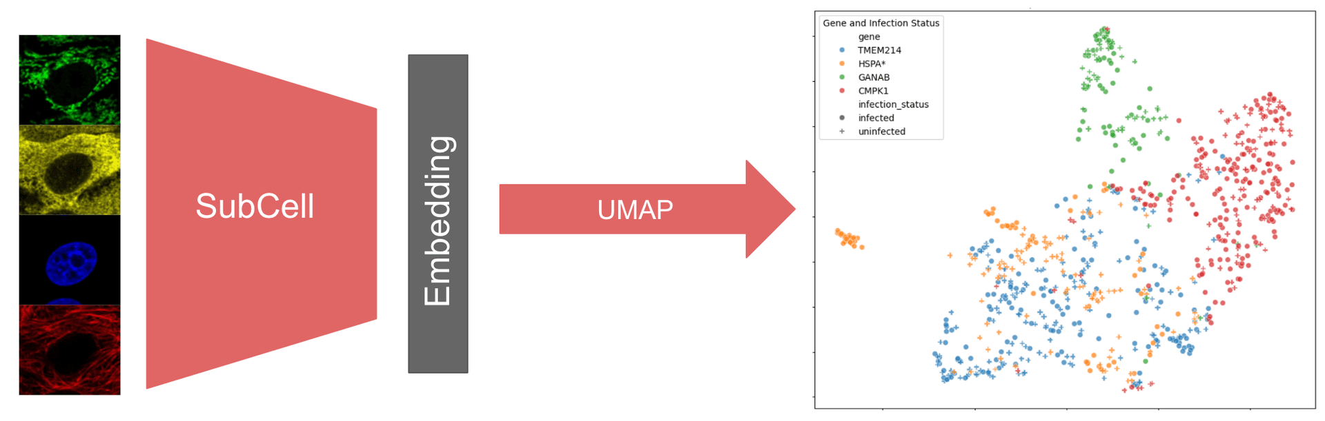
In machine learning (ML), embeddings are simplified representations of the input data that encode the key features of the data. Embeddings are a fundamental part of many ML models’ operation since they enable the model to learn complex patterns within the data and represent those patterns in a more compact way. In addition to aiding computation, embeddings themselves can be valuable model outputs. Models that take in data and output embeddings are called encoder models. Encoder models are particularly valuable for analyzing large, complex datasets, where identifying patterns directly from the raw data can be challenging. Since embeddings are rich representations of the data, subsequent ML models can be trained using embeddings from encoder models instead of using the raw data. For example, classifier models can be trained on the output of image encoder models.
Exploring the embedding space can also reveal insights about the underlying raw data. For instance, outliers in the embedding space may indicate anomalies in the input data, or embedding similarity can indicate groupings of the raw data. In either case, exploring the embedding space can be facilitated by further reducing the dimensions of the embeddings to a 2D or 3D space for visual inspection. In this tutorial, the Uniform Manifold Approximation and Projection (UMAP) method will be used to reduce the dimensionality of the embeddings.
Introduction to SubCell
SubCell is a suite of image encoder models developed by Ankit Gupta in Professor Emma Lundberg’s lab. The SubCellPortable Github repository provides code to run the suite of models along with classifier models that were trained on the SubCell embeddings to classify which of 31 different localization categories, such as nucleoli, vesicles, or mitochondria, correspond to a given protein of interest.
Each image encoder model takes as inputs fluorescence microscopy images of cells stained for a protein of interest along with reference markers (nuclei, microtubules, and endoplasmic reticulum) and outputs image embeddings. SubCell models were trained with different combinations of reference markers and each model therefore expects different input channels to run inference. These are summarized in the table below along with the abbreviations used for each model in SubCellPortable. For each set of reference markers, 2 encoder models are available: the "ViT" version was trained with only protein-specific loss, and the "MAE" version was trained with Masked Autoencoder (MAE) Reconstruction Loss, cell-specific and protein-specific losses.
SubCell Model | SubCellPortable Name | Reference Images Required |
|---|---|---|
| DNA-protein | bg | nuclei |
| MT-DNA-protein | rbg | microtubules and nuclei |
| all-channels | rybg | microtubules, ER, and nuclei |
| ER-DNA-Protein | ybg | ER and nuclei |
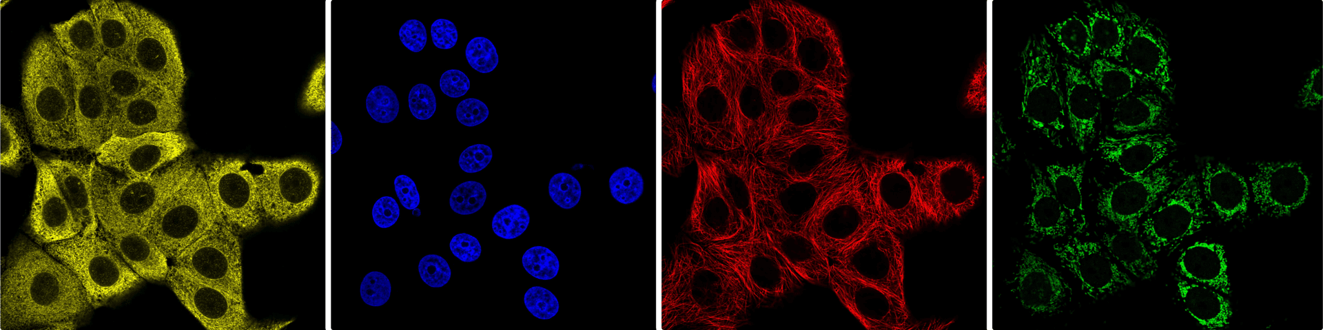
SubCell was trained on individual cell crops from the Human Protein Atlas (HPA) SubCellular data, which includes immunofluorescence of 13,147 proteins of interest and 37 different human cell lines. Below are example field of view images for each of the 4 channels in the 2D HPA data: endoplasmic reticulum (yellow), nucleus (blue), microtubules (red), and protein of interest (green).
This tutorial demonstrates how to run model inference with SubCell. Model inference is the process of feeding input data into a trained machine learning model, in this case a SubCell model, where weights are all learned and frozen, to compute outputs such as embeddings.
SubCell model inference has specific requirements for input data:
- The images must be 2D, so for 3D data, use the max projection along z to create 2D images.
- The resolution of the images must be high enough to segment individual cells and resolve protein patterns.
- Each input image must be of a single cell, so field of view images should segmented into individual cells and each cell cropped from the field of view image and saved as a separate file. Any cell segmentation method may be used for this step.
- Each channel in the cell crop must be saved as a separate PNG file.
- Images must be of 640 x 640 pixels in size with a 80.0885 nm pixel size, rescaling of the image pixel size and resizing of the images may be necessary.
Setup
Google Colab and SubCellPortable must be set up to complete this tutorial.
However, with some modification the same tutorial can be run locally with the demo data provided or with your own data!
If you choose to work locally, to follow best practices, an environment manager should be used. Environment managers
allow the creation of multiple virtual environments, like separate sandboxes, on a computer for installing programs,
like SubCellPortable, without affecting other parts of the system. Virtualenv
is the recommended environment manager for SubCellPortable.
Setup Google Colab
This tutorial is a notebook that can be run within the Google Colab interface.
To start, connect to the T4 GPU runtime hosted for free by Google Colab using the dropdown menu in the upper right
hand corner of this notebook. Using a GPU significantly speeds up running model inference.
Note that this tutorial will use commands written for Google Colab, and some of those commands may need to be modified to work with other computing setups.
Setup SubCellPortable
SubCellPortable is a convenient code wrapper to run the SubCell models in inference along with the provided classifer models in a local environment, or in this case, on Google Colab.
To run SubCellPortable in Google Colab, start by cloning the SubCellPortable repo and navigate to the newly created
SubCellPortable folder using the commands below. The folder will also be present in the file management system in Google
Colab which is accessible by clicking the folder icon on the left hand side bar of this notebook.
# clone the SubCellPortable repo
!git clone https://github.com/CellProfiling/SubCellPortable.git

# navigate the SubCellPortable directory
%cd /content/SubCellPortable
Overview of SubCellPortable
SubCellPortable contains several items in its top level directory, which are described in the table below.
File Name | Description/Purpose |
|---|---|
| models | Subdirectory containing information about models available for inference |
| LICENSE | Licensing information; SubCell is licensed under the MIT License (https://opensource.org/license/mit). |
| README.md | Summary of SubCell usage and requirements |
| config.yaml | Optional file for specifying inference parameters |
| inference.py | Submodule that defines functions for running inference; used in `process.py` |
| models_urls.yaml | Optional file for specifying the URLs for downloading the models |
| path_list.csv | Example of the required file that specifies data location for model inference |
| process.py | Master module for running model inference; call `process.py` to run model inference |
| requirements.txt | List of required packages for running SubCell |
| vit_model.py | Submodule for running vision transformer; used in `process.py` |
The packages required for model inference are listed in requirements.txt and below for convenience.
scikit-image==0.22.0
torch==2.4.1
torchvision==0.19.1
PyYAML==6.0.1
transformers==4.45.1
numpy==1.26.4
pandas==2.2.3
requests==2.32.3
Install those packages using the following. This may take a few minutes, and note that errors in the output dialog will not prevent proceeding with the tutorial as long as the code cell finishes running.
# Install all packages in requirements.txt
!pip install -r requirements.txt
Models Subdirectory
The models subdirectory contains a folder for each of the available models, i.e. ybg or rygb, and in each of those folders, 2 folders mae_contrast_supcon_model and vit_supcon_model correspond to 2 versions of the encoder models that were trained with different loss functions. For each model training, the model_config.yaml file specifies the model location on the machine and the parameters for running the model.
The model_config.yaml file can be manually updated with the absolute path to the model if the model has been
downloaded on the machine. However, it is updated automatically using the models_urls.yaml file whenever the
update_models parameter in process.py is set to True. In this tutorial, a downloaded model will be used, so the
model_config.yaml file will be manually updated before running model inference.
path_list.csv
In SubCellPortable, the path_list.csv file specifies the location of the input cell crops (640 x 640 pixel PNG
files) on the machine and defines output parameters. In path_list.csv, each row corresponds to a cell crop image and
the first 4 columns correspond to the locations of the images for each channel in the following order: microtubule
marker, endoplasmic reticulum (ER) marker, nuclei marker, protein of interest marker, and are referred to as r_image,
y_image, b_image, and g_image, respectively, in SubCellPortable. Depending on the selected model, some of the
image location columns can be left blank. The last 2 columns are output_folder and output_prefix, which specify
where to store the model output and what unique prefix to append to the resulting files for a given cell crop image (see
the Model Outputs section for details on these output files). Every entry in path_list.csv is the
(relative or absolute) path to the corresponding image file on the machine, or in this case, in Google Colab's file
management system. An example path_list.csv file is provided in the repo. Double click on the file to open a preview
in Google Colab. Note the # comments out the cell, so the first row that names the columns all have #.
Use Case
SubCell can be used for a wide variety of applications that involve exploring protein localization patterns. In this tutorial, changes to protein localization patterns in vitro following infection with severe acute respiratory syndrome coronavirus-2 (SARS-CoV-2) will be explored building off of the study 'Subcellular mapping of the protein landscape of SARS-CoV-2 infected cells for target-centric drug repurposing' by JM Kaimal et al. SARS-CoV-2 infection causes COVID-19 in humans, and understanding how infection impacts cells in vitro can elucidate mechanisms of action that reveal potential preventative and treatment options for COVID-19.
In the study referenced above, the authors used antibodies from the Human Protein Atlas for immunofluorescence imaging to analyze changes in host protein levels and subcellular localization upon SARS-CoV-2 infection. Using 602 antibodies targeting 662 genes, the team conducted immunostaining in infected and non-infected Vero E6 cells with markers for SARS-CoV-2 infection, endoplasmic reticulum, nucleus, and protein of interest. Images were acquired with 9 fields of view and 3 z planes per protein of interest. The images were analyzed using the Covid Image Annotator tool on the ImJoy platform, where a DPNUnet model segmented cells and identified infected vs. non-infected cells based on staining of the SARS-CoV-2 nucleocapsid protein. Through laborious, manual image annotation, they identified 97 proteins that exhibited either spatial redistribution or altered abundance between infected and non-infected cells. In the future, SubCell or a similar model may be able to replace this time-intensive process.
The available raw data is not in the required format for SubCell. The images were acquired with Opera Phenix high-content microscope (PerkinElmer) in confocal mode with a 63X water objective with a binning factor of 2 resulting in an effective pixel size of 205 nm, and the data is of the full field of view images including multiple cells per image.
To prepare this data for SubCell, images were segmented into individual cell crops, rescaled to an 80 nm pixel size,
resized to 640 x 640 pixels in size with the cell located at the center of the cell crop image, and each channel (ER,
nuclues, and protein) was saved as its own PNG file. These PNG files do not include SARS-CoV-2 virus staining. Instead,
the infection status is indicated with a 1 for infected and 0 for uninfected in the third column of a metadata file,
single_cell_metadata.csv, which also includes corresponding information on the antibody used in each well to label the
relevant protein of interest.
Only a subset of data for 4 proteins will be examined in this tutorial. A table of the genes associated with the antibody stain along with the well IDs for the images, and observed localization changes is found below.
Gene | Well | Observed Change |
|---|---|---|
| TMEM214 | 1_E3 | None |
| HSPA* | 2_H10 | Spatial, Intensity up |
| GANAB | 4_G11 | Spatial |
| CMPK1 | 6_F5 | Spatial |
Download Data, Metadata, and Models for the Tutorial
Since the data contains ER and nuclei reference markers, a ybg model will be used for inference. In this tutorial, the "MAE" version of the ybg model will be used, but please refer to the SubCell preprint paper for guidance on which model version is most appropriate for a given use case. To examine changes in localization, one of the provided classifier models will be used.
Image data, the metadata file single_cell_metadata.csv, a prepared path_list.csv, ybg model, and a classifier
model can be downloaded as a zip file using the below code or manually from this link.
# download zip file containing data, models, and path_list.csv
!gdown --fuzzy https://drive.google.com/file/d/1-Vym0Yr2ZGnqRX4UsIorDH1vXBqzSNKF/view?usp=sharing
A file, subcell_tutorial_data_models.zip should now appear in the file manager under the SubCellPortable directory. To unzip this file and replace the example path_list.csv file in SubCellPortable with one prepared for this tutorial, use the following. This may take a few minutes.
# unzip the file and replace the path_list.csv example file with the one in the zip file
!unzip -o subcell_tutorial_data_models.zip
Unzipping the file, creates 4 entities:
imagesfolder with 3 subfolders,er,nucleus, andprotein, containing the images corresponding to each channel.subcell_encoder_model.pth(332 MB) file is the image encoder model.subcell_classifier_model.pth(3 MB) file is the classifier model.path_list.csvis the prepared metadata file for the images.
In path_list.csv, the image locations are relative paths, the output folder is called output for all images, and the
unique output prefixes were defined using information from single_cell_metadata.csv, where for each cell crop image,
its well, image, and cell ID are combined with infection status ("infected" or "uninfected"). For example, the output
prefix "1_E3_3_25_uninfected" indicates that cell number 25 from the image 3 collected from well 1_E3 was not infected
with SARS-CoV-2. A careful choice of output prefix aids annotation of the resulting UMAPs as will be demonstrated later
in the tutorial.
Run Model Inference
To run inference, the models and data locations must be specified. The downloaded path_list.csv file already specifies
the data locations using relative paths, and the model can be specified with the instructions below.
Specify Model
The paths to the subcell_encoder_model.pth and subcell_classifier_model.pth models must be set in the file /content/SubCellPortable/models/ybg/mae_contrast_supcon_model/model_config.yaml. Double click the link, edit the classifier_paths and encoder_path fields with the locations of the model in Google Colab, and save it (CTRL+S or CMD+S). The updated file is shown below:
classifier_paths:
   - "/content/SubCellPortable/subcell_classifier_model.pth"
encoder_path: "/content/SubCellPortable/subcell_encoder_model.pth"
model_config:
 vit_model:
     hidden_size: 768
     num_hidden_layers: 12
     num_attention_heads: 12
     intermediate_size: 3072
     hidden_act: "gelu"
     hidden_dropout_prob: 0.0
     attention_probs_dropout_prob: 0.0
     initializer_range: 0.02
     layer_norm_eps: 1.e-12
     image_size: 448
     patch_size: 16
     num_channels: 3
     qkv_bias: True
 pool_model:
     dim: 768
     int_dim: 512
     num_heads: 2
 num_classes: 31
Choose Method for Running Inference
There are 3 options for running SubCellPortable for model inference. This tutorial uses the Option 1 method.
Each option is described below with the same parameters, namely running SubCellPortable with the "MAE" version of the
ybg model; using the model information in the model_config.yaml file instead of downloading the model using the
models_urls.yaml file; creating the optional result.csv output file; and running inference with a GPU (T4 GPU in
Google Colab is used in this tutorial, but use "-1" instead of "0" for CPU compute).
Option 1: Using constants in process.py
If you plan to run SubCell with the same model and parameters, simply edit the constants directly in lines 35-40 in
/content/SubCellPortable/process.py and run model inference with: python process.py
Double click the above link, edit lines 36-40 with the code below, and save it before continuing.
config["model_channels"] = "ybg" # select the ybg model
config["model_type"] = "mae_contrast_supcon_model" # select the model type
config["update_model"] = False # use the model in the models folder
config["create_csv"] = True # create results.csv
config["gpu"] = 0 # use the GPU numbered 0 (use -1 for CPU compute)
The other options are described below for convenience, but skip to the next cell to continue the tutorial.
Option 2: Using flags to specify parameters
Alternatively, you can specify all the model parameters as additional flags when calling python process.py. To see a
list of available parameters, call: python process.py –-help
The available flags along with their arguments are described in the table below.
Flag | Argument | Usage |
|---|---|---|
| --help | N/A | Show the help message that lists optional arguments |
| -c | rybg, rbg, ybg, or bg | Model to be used |
| -t | mae_contrast_supcon_model or vit_supcon_model | Model version to be used; mae_contrast_supcon_model is default |
| -u | True or False | update_model parameter; Sets whether the model should be downloaded using the URL in the models_config.yaml file |
| -csv | True or False | Create results.csv |
| -g | -1, 0, 1, 2, 3 | -1: use CPU; otherwise, GPU ID to use for inference |
An example call that achieves the same result as described above is:
python process.py -c ybg -t mae_contrast_supcon_model -u False -csv True -g 0Option 3: Using the config.yaml file
The final option for running SubCellPortable is to edit the config.yaml file with the desired parameters and simply
call: python process.py
An example config.yaml file is below:
model_channels: "ybg"
model_type: "mae_contrast_supcon_model"
update_model: False
create_csv: True
gpu: 0
Note that the default config.yaml file in SubCellPortable has all of the fields commented out using the # symbol
at the start of each line.
Start Model Inference
Simply run the next code cell to start inference on the data. This may take a few minutes.
# Run Model Inference (Using Option 1 with parameters defined in process.py)
!python process.py
Model Outputs
SubCellPortable has 3 default outputs and 2 optional ones summarized in the table below.
Output | Description | Type |
|---|---|---|
| *_embedding.npy | 1536 dimension embedding vector | Default |
| *_probabilities.npy | Array of weighted probabilities of each subcellular location class | Default |
| *_attention_map | 64x64 PNG thumbnail of the attention map | Default |
| log.txt | Command line interface log from running the model | Optional |
| results.csv | Metadata, probability arrays, and embeddings for all cells | Optional |
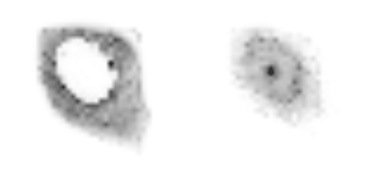
Attention maps are grayscale images that indicate where the model has focused with higher values corresponding to areas where the model has had larger focus. The "MAE" version of the ybg model has 2 attention heads, which like a human observer, appear to focus on the cytosol and nuclei of the cells. An example of an attention map from running the model, which contains the results for each attention head, is shown below.
SubCellPortable has IDs for each localization category. These IDs are referenced in *_probabilities.npy and
result.csv. The localization categories with their corresponding IDs can also be found in
/content/SubCellPortable/inference.py in lines 7-39 under CLASS2NAME. Double click the link to open inference.py
and review the mappings of IDs to localization category if desired.
result.csv is a compilation of metadata, probability arrays, and embeddings for all cells, which is a convenient
collection of data for subsequent analysis.
In result.csv, each row corresponds to one cell, and the columns of result.csv are described below:
Column | Description |
|---|---|
| id | Specified output_prefix |
| top_class_name | Name of the most likely localization class |
| top_class | ID of the most likely localization class |
| top_3_classes_names | Names of the top 3 most likely localization classes |
| top_3_classes | IDs of the top 3 most likely localization classes |
| prob00 - prob30 | Probabilities array for all localization classes |
| feat0000 - feat1535 | 1536 dimension embedding vector |
The rest of this tutorial will describe how to analyze result.csv to explore the embeddings.
Analysis of Model Outputs
The UMAP dimensionality reduction algorithm will be used to enable visualization of the embeddings. Google Colab has
several libraries pre-installed for numerical data analysis and visualization, which will be imported in the notebook,
but it does not have the library for UMAP pre-installed, so to start, install umap-learn with the following.
!pip install umap-learn# Import libraries that come pre-installed in Google Colab
import pandas as pd # data analysis library
import matplotlib.pyplot as plt # visualization library
import seaborn as sns # visualization library
# Import umap-learn library that was installed in the above cell
import umap # dimensionality reduction libraryTo apply UMAP, the embedding vectors need to be read, and to interpret the resulting UMAP, the reduced embeddings need
to be annotated with the gene labeled and the infection status of the cells. The result.csv file can be read and
modified using the code below to append 2 additional annotation columns, one for the gene and one for the infection
status of the cell.
# read result.csv into a pandas dataframe
df = pd.read_csv("/content/SubCellPortable/result.csv")

# define 'ids' as the id column from `result.csv` (output prefix for a cell)
ids = df["id"]

# add a column 'gene' that captures the well id of the cell (extract just the first 2 elements of the id column)
df["gene"] = ids.str.extract(r'^([^_]+_[^_]+)')[0]

# Convert the well ids to gene names in the 'gene' column
dataset_mapping = {
    '1_E3': 'TMEM214',
    '2_H10': 'HSPA*',
    '4_G11': 'GANAB',
    '6_F5': 'CMPK1'
}
df['gene'] = df['gene'].replace(dataset_mapping)

# add a column 'infection_status' that indicates whether the cell was infected or unifected (extract the last element of the id)
df["infection_status"] = ids.str.extract(r'([^_]+)$')[0]
The UMAP should only be performed on the embedding vectors in result.csv, so next, extract the columns containing the
embedding vectors and perform UMAP on those vectors. For more information on the UMAP library, refer to
this documentation.
# extract the embedding vectors (all columns that start with 'feat')
features = df.loc[:, df.columns.str.startswith("feat")]

# apply UMAP to the embedding vectors
reducer = umap.UMAP()
reduced_features = reducer.fit_transform(features)
To understand how the data has transformed with each modification, optionally display the data in df, features, and
reduced_features with the 3 code cells below.
# OPTIONAL: view the data in df = result.csv with 2 new columns ('gene', 'infection_status')
df# OPTIONAL: view the data in features = 1536 dimension embeddings
features# OPTIONAL: view the data in reduced_features = 2 column array with one row for each embedding
reduced_featuresWith the UMAP performed, the reduced embeddings can be visualized in 2D using matplotlib.
# Create a dataframe for the reduced embeddings along with their annotations
umap_df = pd.DataFrame(reduced_features, columns=["UMAP1", "UMAP2"])
umap_df["gene"] = df["gene"]
umap_df["infection_status"] = df["infection_status"]

# Use matplotlib and seaborn to visualize the results as a UMAP
plt.figure(figsize=(10, 8))
sns.scatterplot(
    data=umap_df,
    x="UMAP1",
    y="UMAP2",
    hue="gene",
    style="infection_status",
    palette="tab10",  # Set palette for unique colors per dataset
    markers=["o", "P"],  # Shapes for infected and uninfected
    alpha=0.7
)

# Add legend and title
plt.legend(title="Gene and Infection Status")
plt.title("UMAP Projection of Feature Data")
plt.show()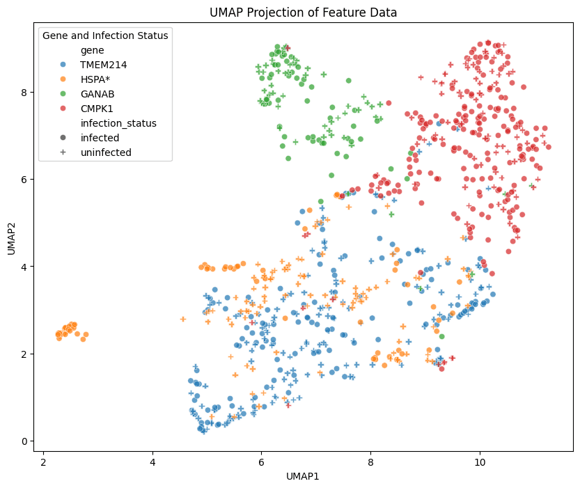
While scientific interpretation of the UMAP is not the focus of this tutorial, below is the summary table of the changes observed in the referenced study for each of the genes.
Gene | Observed Change |
|---|---|
| TMEM214 | None |
| HSPA* | Spatial, Intensity up |
| GANAB | Spatial |
| CMPK1 | Spatial |
At a glance, the distribution of blue circles (infected) and crosses (uninfected) that correspond to the TMEM214 gene seem to have relatively more overlap than the distributions of the other 3 genes' reduced embeddings. This is in line with the observation in the study of no change to protein localization pattern between the infected and uninfected cells in the TMEM214 group, whereas, for the other 3 genes, changes were observed.
In the above UMAP, each datapoint corresponds to one cell in the data, and the spread of the datapoints for a given condition represents the variation present in the underlying image data. However, there are other methods of grouping data for a UMAP. To illustrate another way of grouping data, in the following sections, UMAP will be done on the averaged embeddings for each condition (i.e. uninfected cells with proteins from the GANAB gene labeled).
# Ensure 'feat' is a list of column names that start with "feat"
feat_columns = [col for col in df.columns if col.startswith("feat")]

# Group by 'dataset' and 'infection_status' and calculate the mean for only "feat" columns
averaged_feat = df.groupby(['gene', 'infection_status'])[feat_columns].mean().reset_index()
To understand how the data has transformed, optionally display the data in averaged_feat with the code cell below. Now
there are only 8 rows for the 8 cases in the data.
# OPTIONAL: view the data in averaged_feat = 8 row array of averaged embeddings
averaged_feat
In these next cells, UMAP will be performed on the averaged embeddings, and the resulting reduced embeddings will be visualized using the same approach as used above.
# apply UMAP to the averaged embedding vectors
reduce_avg = umap.UMAP()
avg_embedding = reduce_avg.fit_transform(averaged_feat.iloc[:, 2:]) # using iloc to select the columns with the embeddings# Create a dataframe for the UMAP results and labels
umap_avg = pd.DataFrame(avg_embedding, columns=["UMAP1", "UMAP2"])
umap_avg["gene"] = averaged_feat["gene"]
umap_avg["infection_status"] = averaged_feat["infection_status"]# Plotting
plt.figure(figsize=(10, 8))
sns.scatterplot(
data=umap_avg,
x="UMAP1",
y="UMAP2",
hue="gene",
style="infection_status",
palette="tab10", # Set palette for unique colors per dataset
markers=["o", "P"], # Shapes for infected and uninfected
alpha=0.7
)
# Add legend and title
plt.legend(title="Gene and Infection Status")
plt.title("UMAP Projection of Feature Data")
plt.show()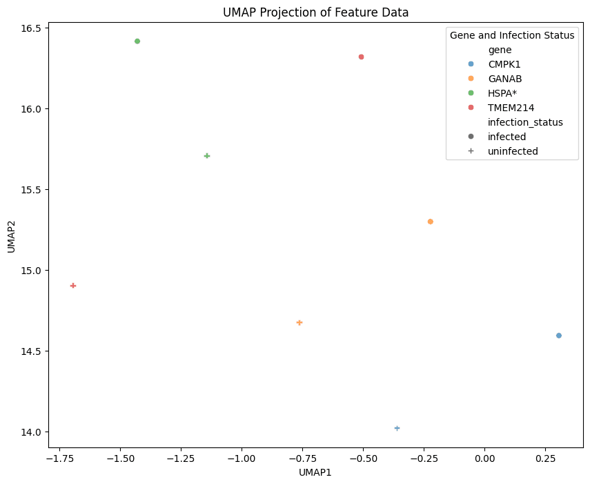
These average embeddings may not look exactly as expected, and the visualization above is for illustrative purposes only to demonstrate an example of how to average embeddings and visualize the resulting UMAP. Averaging embeddings before applying UMAP can obscure the natural variation between individual datapoints by collapsing unique features into a single averaged representation, potentially masking important group-specific patterns or clusters that UMAP would otherwise capture. UMAP approximates the underlying topological manifold of the dataset in a lower-dimensional space. Because this tutorial uses only a small subset of the data (4 genes out of a total of 662), the resulting embeddings do not represent the full variation and complexity of the manifold of the full dataset. As a result, patterns or groupings seen here may not generalize to the entire dataset and could be misleading if interpreted as comprehensive. In addition, when simplifying the data through averaging, multiple methods should be explored (e.g. averaging across images, averaging across genes, etc.), and whenever using strategies like UMAP, the effect of changes to parameters should be explored before the results are trusted for scientific evaluation. Check out this example of exploring the parameter space from the UMAP-learn documentation for more information.
The above steps and code can be modified to analyze the full dataset or your own data of interest for rigorous scientific inquiry.
Summary
Image embeddings are vector outputs of image encoder models that represent the essential features or patterns of images. Since embeddings capture the key features of the image data, images that are visually or categorically similar will have embeddings that are similar to each other in the embedding space. Embeddings can be used for computation or to train downstream models like classifiers, but embeddings themselves can also be valuable as model outputs. Exploring the embedding space can be facilitated by further reducing the dimensions of the embeddings to a 2D or 3D space for visual inspection using algorithms like UMAP.
SubCell is an image encoder model developed by Ankit Gupta in Professor Emma Lundberg’s lab. This model takes in fluorescence microscopy images of cells and outputs image embeddings along with predictions of the localizations of the proteins in the images from a classifier model that was trained on SubCell embeddings. SubCell can be used for a wide variety of applications that involve exploring protein localization patterns. In this tutorial, data from the study "Subcellular mapping of the protein landscape of SARS-CoV-2 infected cells for target-centric drug repurposing" by JM Kaimal et al were explored using SubCellPortable to examine how embeddings could represent changes to protein localization patterns in vitro following infection with SARS-CoV-2.
Contact and Acknowledgments
For issues with this tutorial please contact virtualcellmodels@chanzuckerberg.com.
Special thank you to Ankit Gupta, William Leineweber, and Frederic Ballllosera from Professor Emma Lundberg's lab for their consultation on this tutorial.
References
- "SubCell: Vision foundation models representing cell biology" by Ankit Gupta et al
- "Subcellular mapping of the protein landscape of SARS-CoV-2 infected cells for target-centric drug repurposing" by JM Kaimal et al
Responsible Use
We are committed to advancing the responsible development and use of artificial intelligence. Please follow our Acceptable Use Policy when engaging with our services.
Should you have any security or privacy issues or questions related to the services, please reach out to our team at security@chanzuckerberg.com or privacy@chanzuckerberg.com respectively.